6.4 Gráfica de validación

La gráfica de validación compara las estimaciones directas, las del modelo y las ajustadas por benchmarking. En este código se genera un gráfico utilizando la librería ggplot2 de R. Primero, se seleccionan las variables correspondientes a las estimaciones del modelo para la categoría de empleo correspondiente ( Ocupado, Desocupado e Inactivo), se transforman los datos a formato largo con la función gather() y se asignan etiquetas para las distintas estimaciones. Luego, se crea un data.frame con los límites de los intervalos de confianza para las estimaciones obtenidas directamente de la encuesta. Finalmente, se utiliza la función ggplot() para graficar los datos, agregando una capa para mostrar los intervalos de confianza y otra capa para mostrar los valores de las estimaciones.

Ocupado

temp_ocupado <- data_plot %>% select(dam,nd, starts_with("Ocupado"))


temp_ocupado_1 <- temp_ocupado %>% select(-Ocupado_low, -Ocupado_upp) %>%
  gather(key = "Estimacion",value = "value", -nd,-dam) %>% 
  mutate(Estimacion = case_when(Estimacion == "Ocupado_mod" ~ "Modelo de área",
                                Estimacion == "Ocupado_Bench" ~ "Modelo de área (bench)",
                                Estimacion == "Ocupado"~ "Directo"))
lims_IC_ocupado <-  temp_ocupado %>%
  select(dam,nd,value = Ocupado,Ocupado_low, Ocupado_upp) %>% 
  mutate(Estimacion = "Directo")

p_ocupado <- ggplot(temp_ocupado_1,
            aes(
              x = fct_reorder2(dam, dam, nd),
              y = value,
              shape = Estimacion,
              color = Estimacion
            )) +
  geom_errorbar(
    data = lims_IC_ocupado,
    aes(ymin = Ocupado_low ,
        ymax = Ocupado_upp, x = dam),
    width = 0.2,
    linewidth = 1
  )  +
  geom_jitter(size = 3)+
  labs(x = "Dam", title = "Ocupado")

Desocupado

temp_Desocupado <- data_plot %>% select(dam,nd, starts_with("Desocupado"))


temp_Desocupado_1 <- temp_Desocupado %>% select(-Desocupado_low, -Desocupado_upp) %>%
  gather(key = "Estimacion",value = "value", -nd,-dam) %>% 
  mutate(Estimacion = case_when(Estimacion == "Desocupado_mod" ~ "Modelo de área",
                                Estimacion == "Desocupado_Bench" ~ "Modelo de área (bench)",
                                Estimacion == "Desocupado"~ "Directo"))
lims_IC_Desocupado <-  temp_Desocupado %>%
  select(dam,nd,value = Desocupado,Desocupado_low, Desocupado_upp) %>% 
  mutate(Estimacion = "Directo")

p_Desocupado <- ggplot(temp_Desocupado_1,
                    aes(
                      x = fct_reorder2(dam, dam, nd),
                      y = value,
                      shape = Estimacion,
                      color = Estimacion
                    )) +
  geom_errorbar(
    data = lims_IC_Desocupado,
    aes(ymin = Desocupado_low ,
        ymax = Desocupado_upp, x = dam),
    width = 0.2,
    linewidth = 1
  )  +
  geom_jitter(size = 3)+
  labs(x = "Dam", title = "Desocupado")

Inactivo

temp_Inactivo <- data_plot %>% select(dam,nd, starts_with("Inactivo"))


temp_Inactivo_1 <- temp_Inactivo %>% select(-Inactivo_low, -Inactivo_upp) %>%
  gather(key = "Estimacion",value = "value", -nd,-dam) %>% 
  mutate(Estimacion = case_when(Estimacion == "Inactivo_mod" ~ "Modelo de área",
                                Estimacion == "Inactivo_Bench" ~ "Modelo de área (bench)",
                                Estimacion == "Inactivo"~ "Directo"))
lims_IC_Inactivo <-  temp_Inactivo %>%
  select(dam,nd,value = Inactivo,Inactivo_low, Inactivo_upp) %>% 
  mutate(Estimacion = "Directo")

p_Inactivo <- ggplot(temp_Inactivo_1,
                       aes(
                         x = fct_reorder2(dam, dam, nd),
                         y = value,
                         shape = Estimacion,
                         color = Estimacion
                       )) +
  geom_errorbar(
    data = lims_IC_Inactivo,
    aes(ymin = Inactivo_low ,
        ymax = Inactivo_upp, x = dam),
    width = 0.2,
    linewidth = 1
  )  +
  geom_jitter(size = 3)+
  labs(x = "Dam", title = "Inactivo")

p_ocupado/p_Desocupado/p_Inactivo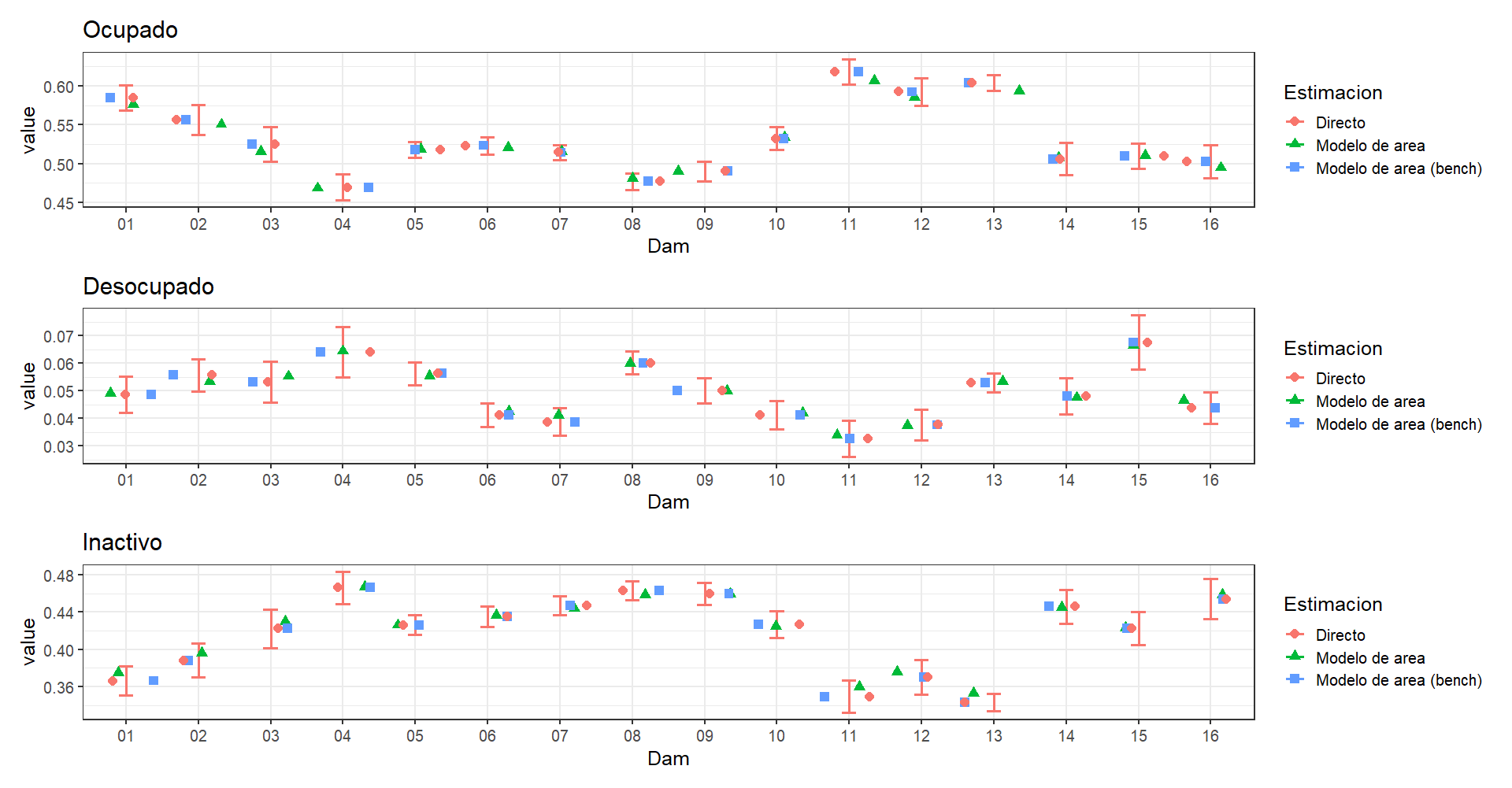

rm(list = ls())
knitr::opts_chunk$set(warning = FALSE, 
                      message = FALSE,
                      cache = TRUE)
library(kableExtra)
tba <- function(dat, cap = NA){
  kable(dat,
      format = "html", digits =  4,
      caption = cap) %>% 
     kable_styling(bootstrap_options = "striped", full_width = F)%>%
         kable_classic(full_width = F, html_font = "Arial Narrow")
}