U1 <- c("Erik", "Sharon")
N1 <- length(U1)
U2 <- c("Yves", "Ken", "Leslie")
N2 <- length(U2)5 Stratified sampling
Stratification is one of the most widespread and widely used techniques in sampling because it has statistical and administrative features that make it attractive: it allows subpopulations to be handled, increases the efficiency of estimates, and contributes to the efficient administration of large surveys.
Valliant et al. (2000)
On some occasions, the characteristic of interest tends to take different average values across population subgroups. In some sense, if the population behaves differently in these subgroups, it is possible to improve the precision of the estimates by taking independent samples in each population subgroup. This is intuitive when there is substantial variability between subgroups, but the variability within them is constant.
In general, when the sampling frame contains auxiliary information that allows the population to be divided into \(H\) subgroups with the objective of selecting a sample in each subgroup, the sampling strategy is said to use a stratified sampling design, and the subgroups formed before information collection are called strata. Note the difference from population subgroups called domains, where the partition of the population is made after the information has been collected.
We often have additional information that helps us design the sampling strategy. When this information refers to each element’s membership in a subgroup, we can apply a strategy that uses a stratified sampling design. It is not only the availability of this auxiliary information that leads us to use a stratified sampling design; in addition: - The variable of interest takes different average values in different subpopulations. - In one way or another (logistical and/or data-collection process), it is better to stratify and divide the population into partitions. Lehtonen and Pahkinen (2003) state that some typical stratification variables are regional (municipality, state, or province), demographic (gender or age group), and socioeconomic (income group). Previous censuses may contain this valuable information.
The need to stratify1 the population arises for one or more of the following reasons: - Administrative reasons. Some sampling frames already have the population divided into naturally formed subgroups. - The goal is to guarantee that the selected sample is representative with respect to population behavior according to the auxiliary information. When selecting a simple random sample from a population of people, it could happen that the selected sample includes no men. - Highly precise estimates are required, disaggregated for each subpopulation. Increase the sample size in the less represented strata. - Lower cost. Different operating schemes for different strata. Mail surveys for large firms. Smaller sample sizes in tolerance zones or areas where public order is difficult to manage. - Reduction of variance in estimation. People of different ages with different blood pressures (stratify by age groups). The variance is reduced because the strata are internally homogeneous but heterogeneous among themselves.
The objective of the stratified design is to give a particular treatment to each subgroup, whether for economic, administrative, or logistical reasons. It is essential to delimit the subgroups well in the design stage. For example, in a study within a university, if the goal is to find out how many hours students spend in front of a computer, it is not a good idea (a technical flaw) to divide the population by courses, because courses do not provide a partition of the population, since the same students may be in different courses.
5.1 Theoretical foundations
Suppose that the sampling frame makes it possible to know the membership of each element of population \(U\) in \(H\) separate population subgroups \(U_h\) (\(h=1,2,\ldots,H\)), also called strata. These are defined as groups of mutually exclusive elements. Each element can belong to one and only one stratum. Thus, - \(\bigcup_{h=1}^H U_h=U\) - \(U_h\bigcap U_i = \emptyset \ \ \ \ \ \ \ h\neq i\)
Each stratum \(U_h\) has size \(N_h\); therefore, \[ \sum_{h=1}^HN_h=N \]
With the population divided into \(H\) strata, the objective remains to estimate the following population parameters - The population total, \[ t_y=\sum_{k \in U}y_k=\sum_{h=1}^H\sum_{k\in U_h}y_k=\sum_{h=1}^Ht_{yh} \] where \(t_{yh}=\sum_{k\in U_h}y_k\). - The population mean, \[ \bar{y}=\frac{\sum_{k \in U}y_k}{N}=\frac{1}{N}\sum_{h=1}^H\sum_{k\in U_h}y_k=\frac{1}{N}\sum_{h=1}^HN_h\bar{y}_h \] where \(\bar{y}_h=\dfrac{1}{N_h}\sum_{k\in U_h}y_k\).
Sampath (2001) states that depending on the nature of the strata, different sampling strategies can be used in different strata. Thus, in the absence of auxiliary information, a simple random strategy may be used in some strata, while for those subgroups whose sampling frame allows continuous auxiliary information to be known, it is possible to apply a sampling strategy proportional to size, and even for those subgroups where, by logistical or technical obligation, a census must be applied.
It is important to clarify that the selection of the \(H\) samples is carried out independently in each stratum.2 Thus, the random sample \(S\)3 is defined by \[ S=\bigcup_{h=1}^HS_h. \]
In particular, if the selected sample is \(s\), then \[ s=\bigcup_{h=1}^Hs_h. \]
Note that if the sample size in each stratum is equal to \(n_h\), then the size of the sample selected through a stratified sampling design is \[ n=\sum_{h=1}^Hn_h. \]
Thus, for each stratum \(h \ \ \ h=1,\ldots,H\), there is a set of all possible samples denoted as the support of stratum \(h\), or \(Q_h\). Each of the supports \(Q_h\) induces the definition of the general support as follows \[ Q^H=\prod_{h=1}^HQ_h. \]
where \(\prod\) denotes the Cartesian product operator4. The cardinality of each support \(Q_h\) depends on the sampling design used to select the sample in stratum \(h\). Thus, \[ \#Q^H=\prod_{h=1}^H\#Q_h. \]
Of course, the stratified sampling design is a genuine sampling design, as stated in the following results.
TipResult
Let \(p_1(s_1),p_2(s_2),\ldots,p_H(s_H)\) be the sampling designs used in each stratum \(h \ \ \ h=1,\ldots,H\). Then the stratified sampling design is defined as \[ p(s)=\prod_{h=1}^Hp_h(s_h) \tag{5.1}\]
Proof.
We have \[ \begin{align*} p(s)&=Pr(\text{Select $s_1$ from $U_1$, $\cdots$, select $s_H$ from $U_H$,})\\ &=p_1(s_1)\cdots p_H(s_H), \end{align*} \] because the selection process is independent in each stratum.
TipResult
The stratified sampling design satisfies - \(p(s)\geq0\) for every \(s\in Q\) - \(\sum_{s\in Q}p(s)=1\)
Proof.
The first property follows immediately because all expressions in equation 5.1 are greater than or equal to zero. The second property follows by mathematical induction on the number of strata. - If \(H=2\), there are two supports, one for each stratum, \(Q_1\) defined as \[ Q_1=\left\{s_{11},s_{12},\ldots,s_{1H_1}\right\} \] and \(Q_2\) defined as \[ Q_2=\left\{s_{21},s_{22},\ldots,s_{2H_2}\right\} \] such that \[ Q^2=\left\{s_{11}\bigcup s_{21},s_{11}\bigcup s_{22},\ldots,s_{11}\bigcup s_{2H_2},\ldots, s_{1H_1}\bigcup s_{2H_2} \right\} \]
Now, since the selection of the samples is carried out independently, in particular we have \[ p\left(s_{11}\bigcup s_{21}\right)=p(s_{11})p(s_{21}) \]
analogously for the element belonging to the support. Now, \[ \begin{align*} \sum_{s\in Q}p(s)&=p(s_{11})p(s_{21})+p(s_{11})p(s_{22})+\ldots+p(s_{11})p(s_{2H_2})+\\ &\ldots+p(s_{1H_1})p(s_{21})+p(s_{1H_1})p(s_{22})+\ldots+p(s_{1H_1})p(s_{2H_2})\\ &=p(s_{11})[\underbrace{p(s_{21})+p(s_{22})+\ldots+p(s_{2H_2})}_{1}]+\\ &\ldots+p(s_{1H_1})[\underbrace{p(s_{21})+p(s_{22})+\ldots+p(s_{2H_2})}_{1}]\\ &=p(s_{11})+\ldots+p(s_{1H_1})\\ &=1 \end{align*} \] - If \(H=k\), suppose that \[ \sum_{s\in Q^k}p(s)=1 \] where \[ Q^k=\left\{\bigcup_{h=1}^ks_h\ \ \ | \ \ s_h\in Q_h\right\}. \] - If \(H=k+1\), there are \(k+1\) supports such that \[ \begin{split} Q_1&=\left\{s_{11},s_{12},\ldots,s_{1H_1}\right\}\\ \vdots\\ Q_k&=\left\{s_{k1},s_{k2},\ldots,s_{kH_k}\right\}\\ Q_{k+1}&=\left\{s_{k+1,1},s_{k+1,2},\ldots,s_{k+1,H_{k+1}}\right\} \end{split} \] Consequently, we have \[ \begin{align*} \sum_{s\in Q}p(s)&=p(s_{k+1,1})\left[\underbrace{\sum_{s\in Q^k}p(s)}_{1}\right] +\ldots+p(s_{k+1,1H_{k+1}})\left[\underbrace{\sum_{s\in Q^k}p(s)}_{1}\right]\\ &=p(s_{k+1,1})+\ldots+p(s_{k+1,H_{k+1}})\\ &=1 \end{align*} \]
5.1.1 Estimation in stratified sampling
If one of the purposes of stratification is to obtain more precise estimates, it is natural to ask what form the estimators take and how to define them across strata; furthermore, what form does the variance of the estimator in the strata and its estimated variance take? The following results answer these questions.
TipResult
If \(\hat{t}_{yh}\) unbiasedly estimates the total of the characteristic of interest \(t_{yh}\) for population subgroup \(h\) with variance equal to \(Var(\hat{t}_{yh})\), then an unbiased estimator for the population total \(t_y\) is given by \[ \hat{t}_y=\sum_{h=1}^H\hat{t}_{yh} \]
which has variance equal to \[ Var(\hat{t}_y)=\sum_{h=1}^HVar(\hat{t}_{yh}) \]
Proof.
Since \(\hat{t}_{yh}\) is unbiased, we have \[ \begin{align*} E\left(\sum_{h=1}^H\hat{t}_{yh}\right)&=\sum_{h=1}^HE\left(\hat{t}_{yh}\right)\\ &=\sum_{h=1}^Ht_{yh}=t_y \end{align*} \]
On the other hand, using the independence of sample selection in each stratum,
\[ \begin{align*} Var\left(\sum_{h=1}^H\hat{t}_{yh}\right)&=\sum_{h=1}^HVar\left(\hat{t}_{yh}\right)+ \sum_{h=1}^H\sum_{i=1}^H\underbrace{Cov\left(\hat{t}_{yh},\hat{t}_{yi}\right)}_{0}\\ &=\sum_{h=1}^HVar(\hat{t}_{yh}) \end{align*} \]
TipResult
If \(\widehat{Var}(\hat{t}_{yh})\) unbiasedly estimates \(Var(\hat{t}_{yh})\), then an unbiased estimator for \(Var(\hat{t}_{y})\) is given by
\[ \widehat{Var}(\hat{t}_{y})=\sum_{h=1}^H\widehat{Var}(\hat{t}_{yh}) \]
Proof.
The proof is immediate from unbiasedness in each of the strata.
5.1.2 The Horvitz-Thompson estimator
TipResult
For the stratified sampling design, the Horvitz-Thompson estimator, its variance, and its estimated variance are given by:
\[ \hat{t}_{y,\pi}=\sum_{h=1}^H \hat{t}_{yh,\pi} \] \[ Var_{ST}(\hat{t}_{y,\pi})=\sum_{h=1}^H Var_{p_h}(\hat{t}_{yh,\pi}) \] \[ \widehat{Var}_{ST}(\hat{t}_{y,\pi})=\sum_{h=1}^H \widehat{Var}_{p_h}(\hat{t}_{yh,\pi}) \]
where \[ \hat{t}_{yh,\pi}=\sum_{k\in S_h}\dfrac{y_k}{\pi_k} \] Here \(Var_{p_e}(\hat{t}_{yh,\pi})\) is the variance of \(\hat{t}_{yh,\pi}\) in the \(h\)-th stratum, and \(\widehat{Var}_{p_h}(\hat{t}_{yh,\pi}\) is the estimate of \(Var_{p_h}(\hat{t}_{yh,\pi})\) in the \(h\)-th stratum.
NoteExample
Our example population \(U\), given by
\[U=\{\textbf{Yves, Ken, Erik, Sharon, Leslie}\}\]
is divided into two strata as follows
\[U_1=\{\textbf{Erik, Sharon}\}\]
and the second composed of:
\[U_2=\{\textbf{Yves, Ken, Leslie}\}\]
In the first stratum, a random sample of size \(n_1=1\) is selected according to a simple random sampling design without replacement. On the other hand, in the second stratum, a sample of size \(n_2=2\) is selected according to the following sampling design
\[ p_2(s)= \begin{cases} 1/4, &\text{if $s=\{\text{Yves, Ken}\}$},\\ 1/4, &\text{if $s=\{\text{Yves, Leslie}\}$},\\ 1/2, &\text{if $s=\{\text{Ken, Leslie}\}$.} \end{cases} \]
Carry out the lexical-graphic calculation to verify the unbiasedness of the Horvitz-Thompson estimator for all possible samples of size \(n=3\). Define the supports \(Q_1\) and \(Q_2\), as well as the general support \(Q^2\) for each stratum.
In the following sections, the stratified designs most commonly used in practice will be studied.
5.2 Stratified random sampling design
Like simple random sampling without replacement, the stratified random sampling design (STR-SRS) is the simplest of the stratified designs. In this particular case, a simple random sample is selected in each stratum so that the selections are independent. This sampling design is used when the variability of the characteristic of interest within the strata is similar; in other words, when the behavior of the characteristic of interest inside the strata is known to be homogeneous. However, it is also used when no continuous auxiliary information is available that would allow sampling designs, in each stratum, to improve the efficiency of a simple random sample.
In each stratum \(h\), a simple random sample without replacement of size \(n_h\) is selected independently from the stratum population of size \(N_h\). Although the simple random sampling design is used as the final method for selecting elements, overall the stratified design can be dramatically more efficient than using a simple random sampling design without dividing the population.
ImportantDefinition
For fixed sample sizes in each stratum, denoted as \(n_1,\ldots,n_H\), a sampling design is said to be stratified simple random without replacement if the probability of selecting a sample of size \(n\) is given by \[ p(s)= \begin{cases} \prod_{h=1}^H\frac{1}{\binom{N_h}{n_h}}, &\text{if $\sum_{h=1}^Hn_h=n$}\\ 0, &\text{otherwise} \end{cases} \]
Note that \(\sum_{s\in Q^H}p(s)=1\) because \(\#Q^H=\prod_{h=1}^H\binom{N_h}{n_h}\).
5.2.1 Selection algorithms
When selecting the simple random samples without replacement in each stratum, it is possible to use the sampling algorithms given in Chapter 3, so that the following steps must be carried out. - Separate the population into \(H\) subgroups or strata by means of the population characterization based on auxiliary information. - In each stratum, select a simple random sample without replacement. The algorithms used to select the sample within each stratum may be the negative coordination method or Fan et al. (1962)’s selection and rejection method. - Each of the \(H\) selections is carried out independently.
NoteExample
Suppose that our example population \(U\) is partitioned according to the previous section. It is necessary to define the two strata in R so that no element has double membership in any stratum.
R allows operations between data sets. In particular, the union operator is used to verify that the union of the strata gives the example population \(U\). Note that the population size is the sum of the sizes of the two strata.
U <- union(U1, U2)
N <- N1 + N2

U
[1] "Erik" "Sharon" "Yves" "Ken" "Leslie"N[1] 5It has been decided to select a simple random sample without replacement of size \(n_1=1\) from \(U_1\) and a simple random sample without replacement of size \(n_2=2\) from \(U_2\). Thus, the overall sample will have size \(n=n_1+n_2=3\).
sam1 <- sample(N1, 1, replace = FALSE)
U1[sam1]
[1] "Sharon"sam2 <- S.SI(N2, 2)
U2[sam2][1] "Ken" "Leslie"sam <- union(U1[sam1], U2[sam2])
sam[1] "Sharon" "Ken" "Leslie"Of course, it is possible to use the sample function built into the generic R environment, or it is also possible to use the S.SI function from the TeachingSampling package. Regardless of the algorithm used to select the simple random samples without replacement, it is important to note that as many samples have been selected as there are strata in the population.
5.2.2 The Horvitz-Thompson estimator
The sampling strategy is defined through the use of the Horvitz-Thompson estimator. This strategy is the best known, most applied, and most discussed in textbooks. To this end, the following result shows the construction of the inclusion probabilities.
TipResult
For a stratified random sampling design, the first- and second-order inclusion probabilities are given by: \[ \pi_k = \dfrac{n_h}{N_h} \ \ \ \text{if $k\in U_h$} \] \[ \pi_{kl}=\begin{cases} \dfrac{n_h}{N_h}, & \text{if $k=l, k \in U_h$},\\\\ \dfrac{n_h}{N_h}\dfrac{n_h-1}{N_h-1}, & \text{if $k,l \in U_h$},\\\\ \dfrac{n_h}{N_h}\dfrac{n_i}{N_i}, & \text{if $k\in U_h, l\in U_i, i\neq h$}. \end{cases} \] respectively. The covariance of the indicator variables is given by \[ \Delta_{kl}=\begin{cases} \dfrac{n_h}{N_h}\dfrac{N_h-n_h}{N_h}, & \text{if $k=l, k \in U_h$},\\\\ -\dfrac{n_h}{N_h^2}\dfrac{(N_h-n_h)}{(N_h-1)}, & \text{if $k,l \in U_h$},\\\\ 0, & \text{if $k\in U_h, l\in U_i, i\neq h$}. \end{cases} \]
Proof.
Let \(k\in U_h\) \[ \begin{align*} \pi_k=Pr(k\in S)&=Pr(k\in S_h)\\ &=Pr(I_k(S_h)=1)\\ &=\dfrac{\binom{1}{1}\binom{N_h-1}{n_h-1}}{\binom{N_h}{n_h}}=\dfrac{n_h}{N_h} \end{align*} \] on the other hand, if \(k,l\in U_h\) \[ \begin{align*} \pi_{kl}&=Pr(k\in S_h\text{ and }l\in S_h)\\ &=Pr(I_k(S_h)=1|I_l(S_h)=1)Pr(I_l(S_h)=1)\\ &=\dfrac{n_h-1}{N_h-1}\dfrac{n_h}{N_h}=\dfrac{n_h}{N_h}\dfrac{n_h-1}{N_h-1} \end{align*} \]
But if \(k\in U_h, l\in U_i, i\neq h\), by the independent selection in strata \(h\) and \(i\), we have
\[ \begin{align*} \pi_{kl}&=Pr(k\in S_h\text{ and }l\in S_i)\\ &=Pr(k\in S_h)Pr(l\in S_i)\\ &=\dfrac{n_h}{N_h}\dfrac{n_i}{N_i} \end{align*} \]
One of the reasons the stratified sampling design is used is that highly precise estimates are desired in the subgroups. Thus, when applying a STR-SRS design, the following result is obtained, which makes it possible to obtain unbiased and precise estimates for each population subgroup.
TipResult
Under a simple random sampling design without replacement in stratum \(h\), an unbiased estimator of the total \(t_{yh}\), its variance, and its estimated variance are given by \[ \hat{t}_{yh,\pi}=\dfrac{N_h}{n_h}\sum_{k\in S_h}y_k \] \[ Var_{SRS}(\hat{t}_{yh,\pi})=\frac{N_h^2}{n_h}\left(1-\frac{n_h}{N_h}\right)S^2_{y_{U_h}} \] \[ \widehat{Var}_{SRS}(\hat{t}_{yh,\pi})=\frac{N_h^2}{n_h}\left(1-\frac{n_h}{N_h}\right)S^2_{y_{S_h}} \] respectively, where \[ S^2_{y_{U_h}}=\frac{1}{N_h-1}\sum_{k\in U_h}(y_k-\bar{y}_{U_h}), \ \ \ \ \quad h=1,\ldots,H. \] the population variance of the characteristic of interest in stratum \(U_h\), and with \[ S^2_{y_{S_h}}=\frac{1}{n_h-1}\sum_{k\in S_h}(y_k-\bar{y}_{S_h}), \ \ \ \ \quad h=1,\ldots,H. \] the sample variance of the values of the characteristic of interest in the random sample from stratum \(S_h\). Note that \(\hat{t}_{yh,\pi}\) is unbiased for the total \(t_{yh}\) of the characteristic of interest \(y\), and that \(\widehat{Var}_{SRS}(\hat{t}_{yh,\pi})\) is unbiased for \(Var_{SRS}(\hat{t}_{yh,\pi})\).
Proof.
By noting that subgroup \(U_h\) can be treated as a separate population, the proof is immediate by following the lines of the proof of Result 3.2.4.
Once the estimates for the population subgroups or strata are available, it follows that the population total \(t_y\) can be estimated using the following result.
TipResult
For a stratified random sampling design, the Horvitz-Thompson estimator of the population total \(t_y\), its variance, and its estimated variance are given by: \[ \hat{t}_{y,\pi}=\sum_{h=1}^H\hat{t}_{yh,\pi}=\sum_{h=1}^H\dfrac{N_h}{n_h}\sum_{k\in S_h}y_k \] \[ Var_{STSI}(\hat{t}_{y,\pi})=\sum_{h=1}^H\frac{N_h^2}{n_h}\left(1-\frac{n_h}{N_h}\right)S^2_{yU_h} \tag{5.2}\] \[ \widehat{Var}_{STSI}(\hat{t}_{y,\pi})=\sum_{h=1}^H\frac{N_h^2}{n_h}\left(1-\frac{n_h}{N_h}\right)S^2_{ys_h} \] respectively. Note that \(\hat{t}_{y,\pi}\) is unbiased for the total \(t_{y}\) of the characteristic of interest \(y\), and that \(\widehat{Var}_{STSI}(\hat{t}_{y,\pi})\) is unbiased for \(Var_{STSI}(\hat{t}_{y,\pi})\).
Proof.
Since \(\hat{t}_{yh,\pi}\) unbiasedly estimates the total \(t_{yh}\) of population subgroup \(h\) with variance given by \(\frac{N_h^2}{n_h}\left(1-\frac{n_h}{N_h}\right)S^2_{yU_h}\), using Results 5.1.3 and 5.1.4 gives the proof immediately.
NoteExample
For our example population \(U\), there are \(\binom{3}{2}\binom{2}{1}=6\) possible samples of size \(n=3\). Carry out the lexical-graphic calculation of the Horvitz-Thompson estimator and verify unbiasedness and the variance.
5.2.3 Estimation of the population mean
One way to know whether there are differences with respect to the values taken by the characteristic of interest in the different strata is to estimate the mean \(\bar{y}_{Uh}\) in subgroup \(U_h\). In fact, the stratified design gains more validity and precision when the average behavior of the characteristic of interest differs in each stratum.
TipResult
Under a simple random sampling design without replacement in stratum \(h\), an unbiased estimator of the mean \(\bar{y}_{Uh}\), its variance, and its estimated variance are given by \[ \hat{\bar{y}}_{Uh,\pi}=\dfrac{1}{n_h}\sum_{k\in S_h}y_k \] \[ Var_{SRS}(\hat{\bar{y}}_{Uh,\pi})=\frac{1}{n_h}\left(1-\frac{n_h}{N_h}\right)S^2_{yU_h} \] \[ \widehat{Var}_{SRS}(\hat{\bar{y}}_{Uh,\pi})=\frac{1}{n_h}\left(1-\frac{n_h}{N_h}\right)S^2_{ys_h} \] respectively. Note that \(\hat{\bar{y}}_{Uh,\pi}\) is unbiased for the stratum mean \(\bar{y}_{Uh}\) of the characteristic of interest \(y\), and that \(\widehat{Var}_{SRS}(\hat{\bar{y}}_{Uh,\pi})\) is unbiased for \(Var_{SRS}(\hat{\bar{y}}_{Uh,\pi})\).
Contrary to the reasoning used in estimating the population total, it is wrong to think as follows:
If an unbiased estimator of the population total $t_y$ is the sum of each of the estimates in the $H$ strata, then an estimator of the population average $\bar{y}_U$ will be an average of the estimated averages in the $H$ strata.The preceding reasoning is intuitive but is wrong for the following reason: \[ \bar{y}_U\neq \dfrac{\bar{y}_{U_1}+\bar{y}_{U_2}+\ldots+\bar{y}_{U_H}}{H} \]
It is easy to see this with our example population \(U\), where the first stratum \(U_1\) has a mean equal to \(\bar{y}_{U_1}=67.5\), and the second stratum \(U_2\) has a mean equal to \(\bar{y}_{U_2}=33.67\). Therefore, \((\bar{y}_{U_1}+\bar{y}_{U_2})/2=50.58\), whereas the true population mean is \(\bar{y}_{U}=47.2\).
TipResult
Under a simple random sampling design without replacement in stratum \(h\), an unbiased estimator of the mean \(\bar{y}_{U}\), its variance, and its estimated variance are given by \[ \hat{\bar{y}}_{U,\pi}=\dfrac{1}{N}\hat{t}_{y,\pi}=\frac{1}{N}\sum_{h=1}^HN_h\hat{\bar{y}}_{Uh,\pi} \] \[ Var_{STSI}(\hat{\bar{y}}_{U,\pi})=\dfrac{Var_{STSI}(\hat{t}_{y,\pi})}{N^2} =\frac{1}{N^2}\sum_{h=1}^H\frac{N_h}{n_h}\left(1-\frac{n_h}{N_h}\right)S^2_{yU_h} \] \[ \widehat{Var}_{STSI}(\hat{\bar{y}}_{U,\pi})=\dfrac{\widehat{Var}_{STSI}(\hat{t}_{y,\pi})}{N^2} =\frac{1}{N^2}\sum_{h=1}^H\frac{N_h}{n_h}\left(1-\frac{n_h}{N_h}\right)S^2_{ys_h} \] respectively. Note that \(\hat{\bar{y}}_{U,\pi}\) is unbiased for the population mean \(\bar{y}_{Uh}\) of the characteristic of interest \(y\), and that \(\widehat{Var}_{SRS}(\hat{\bar{y}}_{U,\pi})\) is unbiased for \(Var_{STSI}(\hat{\bar{y}}_{U,\pi})\).
5.2.3.1 Confidence intervals
In this regard, Lohr (2000) states that a \(100(1-\alpha)%\) confidence interval for the mean of a population is given by
\[ \hat{\bar{y}}_{U,\pi}\pm Z_{1-\frac{\alpha}{2}}\sqrt{Var_{STSI}(\hat{\bar{y}}_{U,\pi})} \]
if some of the following conditions are met - The sample size \(n_h\) in each stratum \(h\) is large. - There is a large number of strata.
If the preceding conditions cannot be satisfied, it is preferable to use the percentile of a Student’s t distribution with \(N-H\) degrees of freedom. Thus, a confidence interval for the population mean is given by
\[ \hat{\bar{y}}_{U,\pi}\pm t_{1-\frac{\alpha}{2},N-H}\sqrt{Var_{STSI}(\hat{\bar{y}}_{U,\pi})} \]
5.2.4 Allocation of sample size
Perhaps the most important part of survey design is determining the sample size. In stratified sampling, under the constraint that the overall sample size is \(n\) and that there are \(H\) fixed strata, the goal is to determine the sample sizes \(n_h\) for each stratum \(h\) in such a way as to guarantee a gain in estimator precision. Lehtonen and Pahkinen (2003) point out that in real sampling studies, which include several characteristics of interest, it is impossible for sample allocation to yield global efficiency gains for every characteristic of interest.
5.2.4.1 Proportional allocation
This type of allocation is chosen when the sample must be representative of the population according to the behavior of the auxiliary information. Lohr (2000) expresses it as follows
When proportional allocation is used, the sample can be viewed as a miniature version of the population.
If the sampling fraction is defined as \(f_h=n_h/N_h\) in stratum \(h\), then when proportional allocation is used, the sampling fraction will be the same for all strata, such that \(f_h=f\). Note that the inclusion probability of any element in the population, \(\pi_k=f_h=f\), is constant and fixed. In this way, each unit in the sample will represent the same number of elements in the population, regardless of the stratum to which it belongs.
ImportantDefinition
A stratified random sampling design has proportional allocation if \[ \frac{n_h}{N_h}=\frac{n}{N}\ \ \ \ \ \ h=1,\ldots,H \]
TipResult
For a stratified random sampling design with proportional allocation, the Horvitz-Thompson estimator of the population total \(t_y\), its variance, and its estimated variance are given by: \[ \hat{t}_{y,\pi}=\dfrac{N}{n}\sum_{k\in S}y_k \] \[ Var_{STSI}(\hat{t}_{y,\pi})=\frac{N^2}{n}\left(1-\frac{n}{N}\right)\sum_{h=1}^H \frac{n_h}{n}S^2_{yU_h} \] \[ \widehat{Var}_{STSI}(\hat{t}_{y,\pi})=\frac{N^2}{n}\left(1-\frac{n}{N}\right)\sum_{h=1}^H \frac{n_h}{n}S^2_{ys_h} \]
Proof.
Observing the relationship in the previous definition, we have \[ \begin{align*} \hat{t}_{y,\pi}&=\sum_{h=1}^H\dfrac{N_h}{n_h}\sum_{k\in S_h}y_k\\ &=\dfrac{N}{n}\sum_{h=1}^H\sum_{k\in S_h}y_k\\ &=\dfrac{N}{n}\sum_{k\in S}y_k \end{align*} \] For the variances, we have \[ \begin{align*} \sum_{h=1}^H\frac{N_h^2}{n_h}\left(1-\frac{n_h}{N_h}\right)S^2_{yU_h}&=\sum_{h=1}^H\frac{N_h^2}{n_h^2}\left(1-\frac{n_h}{N_h}\right)n_hS^2_{yU_h}\\ &=\frac{N^2}{n^2}\left(1-\frac{n}{N}\right)\sum_{h=1}^Hn_hS^2_{yU_h} =\frac{N^2}{n}\left(1-\frac{n}{N}\right)\sum_{h=1}^H\frac{n_h}{n}S^2_{yU_h} \end{align*} \]
5.2.4.2 Neyman allocation
In his 1934 article, Jerzy Neyman discussed the problem of selecting a sample through probabilistic methods versus selecting a convenience sample. In that article, he observed the great advantages of both methods. However, he showed that by separating the population into population subgroups that he called strata and taking simple random samples without replacement, the limits of the confidence interval could be minimized for a fixed sample size. This article was fundamental in the use of stratified sampling around the world.
Neyman addressed the problem of minimizing the variance \(Var_{STSI}(\hat{t}_{y,\pi})\) of the Horvitz-Thompson estimator while fixing the overall sample size \(n\). As Groves et al. (2004) mention, this method produces the smallest variances for the sample mean compared with other sample-size allocation techniques. To carry out this allocation, it is necessary to know the sample sizes in each stratum \(n_h\) such that \(\sum_{h=1}^Hn_h=n\).
TipResult
Under Neyman allocation, the sample size that minimizes (equation 5.2) is given by \[ n_h=n\dfrac{N_hS_{yU_h}}{\sum_{h=1}^HN_hS_{yU_h}} \] where \(S_{yU_h}=\sqrt{S_{yU_h}^2}\).
Proof.
The quantity to minimize is \[ \begin{align*} \sum_{h=1}^H\frac{N_h^2}{n_h}\left(1-\frac{n_h}{N_h}\right)S^2_{yU_h} \end{align*} \] subject to \[ \begin{align*} \sum_{h=1}^Hn_h=n \end{align*} \] The Lagrange equation is written as \[ \mathcal{L}(n_1,\ldots,n_h,\lambda)=\sum_{h=1}^H\frac{N_h^2}{n_h}\left(1-\frac{n_h}{N_h}\right)S^2_{yU_h}-\lambda\left(n-\sum_{h=1}^Hn_h\right) \] setting the partial derivatives to zero gives \[ \begin{align} \frac{\partial\mathcal{L}}{\partial\lambda}&=n-\sum_{h=1}^Hn_h=0\\ \frac{\partial\mathcal{L}}{\partial n_h}&=-\frac{N_h^2}{n_h^2}S^2_{yU_h}+\lambda=0 \end{align} \] From (5.2.28), we have \[ n_h=\frac{N_h}{\sqrt{\lambda}}S_{yU_h} \tag{5.3}\] Replacing in (5.2.27) \[ \begin{align*} \sum_{h=1}^Hn_h=n=\frac{\sum_{h=1}^HN_hS_{yU_h}}{\sqrt{\lambda}} \end{align*} \] Therefore, \[ \sqrt{\lambda}=\frac{1}{n}\sum_{h=1}^HN_hS_{yU_h} \] Finally, replacing in (5.2.29) gives \[ n_h=n\dfrac{N_hS_{yU_h}}{\sum_{h=1}^HN_hS_{yU_h}} \] It is possible to show that the matrix of second partial derivatives is positive definite for the values that satisfy the constraints. Thus, it is concluded that the values of \(n_h\) given by this result minimize the variance of the Horvitz-Thompson estimator under a fixed sample size.
Of course, it is necessary to know the variances of the characteristic of interest in each stratum in order to use this method. With Neyman allocation there are rounding problems; in this case, it is advisable to round to the nearest integer. However, expression (5.2.25) may lead to a situation where \(n_h>N_h\). In this case, a census is conducted in the stratum where the previous relationship occurs, and then the calculation of \(n_h\) is reestablished for the other strata. When a census is conducted in a stratum, due to Neyman allocation or to the logistical design of the survey, that stratum is called a certainty inclusion stratum.
Although using this method can lead to gains in the efficiency of the sampling strategy, Groves et al. (2004) point out the following weaknesses of Neyman allocation: - It does not give good results when estimating proportions, because it requires the proportions to have large differences across strata. In practical life, this situation does not occur in most cases. - By construction, this method works well under the assumption that there is only one characteristic of interest. When working with a multipurpose survey, variance reduction is not achieved for all characteristics of interest included in the study.
5.2.4.3 Optimal allocation
This is a more general method than Neyman allocation. If there is high variability within some stratum, the previous allocation method induces a larger sample size in that stratum. As Lohr (2000) states, in the business sector, for example, the sales of large companies have much greater dispersion than the sales of microenterprises.
However, as in most practical situations, there may be limited financial resources for carrying out the study. Given a budget, if the goal is to minimize the variance of the sampling strategy, another type of allocation must be used. Therefore, defining the following cost function
\[ C=\sum_{h=1}^Hn_hC_h \]
where \(C_h\) is the cost of obtaining the information for the characteristics of interest from a selected element belonging to stratum \(h\), and \(C\) is the total cost of carrying out the study. Then, if the goal is to distribute the selection of elements among the strata given a fixed cost \(C\), in such a way that the variance of the Horvitz-Thompson estimator is minimized, optimal allocation should be used.
TipResult
Under optimal allocation, the sample size that minimizes the cost function is given by \[ n_h=\dfrac{C}{\sqrt{c_h}}\frac{N_hS_{yU_h}}{\sum_{i=1}^HN_i\sqrt{c_i}S_{yU_i}} \]
Proof.
The proof follows immediately by using reasoning similar to the proof of the Neyman allocation result. It is possible to show that the matrix of second partial derivatives is positive definite for the values that satisfy the constraints. Thus, it is concluded that the values of \(n_h\) given by this result minimize the variance of the Horvitz-Thompson estimator under a fixed cost.
The expression for optimal allocation leads to the following conclusions. In a given stratum, a large sample size should be selected if: - The stratum size \(N_h\) is large and information collection in the stratum is cheaper. - The stratum has high dispersion with respect to the study characteristic. In this case, a larger sample is drawn to compensate for heterogeneity within the stratum.
5.2.5 Estimation in domains
Domain estimation is characterized by not knowing in advance whether population units belong to the domain. That is, to know which population units belong to the domain, the measurement process must be carried out. However, there is a similarity between strata and domains: both divide the population into population subgroups. On the one hand, prior knowledge of the membership of population elements in the strata helps improve estimation efficiency in the survey design stage. On the other hand, the price paid for not knowing the membership of population elements in domains is high.
One of the purposes of the stratified sampling design is to reduce the variance of the estimates for the characteristic of interest. This holds when the behavior of the characteristic of interest (as will be seen in the following sections) takes different average values in each stratum. However, in estimating proportions for domains, there is no guarantee that the preceding rule holds.
Now, by multiplying the domain membership variable \(z_{dk}\) given by (3.2.22) by the value of the characteristic of interest \(y_k\), a new variable \(y_{dk}\) is created, given by \(y_{dk}=z_{dk}y_k\). Once constructed, the principles of the Horvitz-Thompson estimator are used to find an unbiased estimator of the total of the characteristic of interest in domain \(U_d\), the absolute size of the domain, and the mean of the characteristic in the domain. Of course, before obtaining estimates at the population level, it is necessary, although not sufficient, to obtain the domain estimates in the strata.
5.2.5.1 Estimation of the total in a domain
TipResult
Under stratified random sampling, the Horvitz-Thompson estimator for the domain total \(t_{yhd}\) in stratum \(h\), its variance, and its estimated variance are given by \[ \hat{t}_{yhd,\pi}=\frac{N_h}{n_h}\sum_{S_h}y_{hdk} \] \[ Var(\hat{t}_{yhd,\pi})=\frac{N_h^2}{n_h}\left(1-\frac{n_h}{N_h}\right)S^2_{y_{dU_h}} \] \[ \widehat{Var}(\hat{t}_{yhd,\pi})=\frac{N_h^2}{n_h}\left(1-\frac{n_h}{N_h}\right)S^2_{y_{ds_h}} \] respectively. \(y_{hdk}\) is the value of the new characteristic \(y_{dk}\) in the \(h\)-th stratum. \(S^2_{y_{dU_h}}\) and \(S^2_{y_{ds_h}}\) denote the variance estimator of the values of the characteristic of interest \(y_{dk}\) in stratum \(U_h\) and in the sample \(s_h\) selected from that stratum, respectively.
TipResult
Under stratified random sampling, the Horvitz-Thompson estimator for the domain total \(t_{yd}\) in the population, its variance, and its estimated variance are given by \[ \hat{t}_{yd,\pi}=\sum_{h=1}^H\frac{N_h}{n_h}\sum_{S_h}y_{hdk} \] \[ Var(\hat{t}_{yd,\pi})=\sum_{h=1}^H\frac{N_h^2}{n_h}\left(1-\frac{n_h}{N_h}\right)S^2_{y_{dU_h}} \] \[ \widehat{Var}(\hat{t}_{yd,\pi})=\sum_{h=1}^H\frac{N_h^2}{n_h}\left(1-\frac{n_h}{N_h}\right)S^2_{y_{ds_h}} \]
Note that in the expression \(S^2_{y_{dU_h}}\), the values involved are those of the characteristic of interest if the element belongs to the domain, and zeros if the element does not belong to the domain; the same occurs with \(S^2_{y_{ds_h}}\). Therefore, the preceding variance expressions will take large values because of the inclusion of zeros; this is the price that must be paid for not knowing element membership in the domains.
5.2.5.2 Estimation of the mean of a domain
TipResult
Under stratified random sampling, the Horvitz-Thompson estimator for the mean of the characteristic of interest in a domain \(\bar{y}_{dU_h}\) in stratum \(h\), its variance, and its estimated variance are given by \[ \hat{\bar{y}}_{dU_h,\pi}=\frac{\hat{t}_{yhd,\pi}}{N_{hd}} \] \[ Var(\hat{\bar{y}}_{dU_h,\pi})=\frac{1}{N_{hd}^2}Var(\hat{t}_{yhd,\pi}) \] \[ \widehat{Var}(\hat{\bar{y}}_{dU_h,\pi})=\frac{1}{N_{hd}^2}\widehat{Var}(\hat{t}_{yhd,\pi}) \]
TipResult
Under stratified random sampling, the Horvitz-Thompson estimator for the mean of the characteristic of interest in a domain \(\bar{y}_{d}\) in the population, its variance, and its estimated variance are given by \[ \hat{\bar{y}}_{d,\pi}=\frac{\hat{t}_{yd,\pi}}{N_{d}} \] \[ Var(\hat{\bar{y}}_{d,\pi})=\frac{1}{N_{d}^2}Var(\hat{t}_{yd,\pi}) \] \[ \widehat{Var}(\hat{\bar{y}}_{d,\pi})=\frac{1}{N_{d}^2}\widehat{Var}(\hat{t}_{yd,\pi}) \]
To use the preceding results, it is necessary to know in advance the value of the absolute size of the domain in each stratum \(N_{hd}\) and the value of the absolute size of the domain in the population \(N_d\).
5.2.5.3 Estimation of the absolute size of a domain
TipResult
Under stratified random sampling, the Horvitz-Thompson estimator for the absolute size of a domain \(N_{hd}\) in stratum \(h\), its variance, and its estimated variance are given by \[ \hat{N}_{hd,\pi}=\frac{N_h}{n_h}\sum_{S_h}z_{dk} \] \[ Var(\hat{N}_{hd,\pi})=\frac{N_h^2}{n_h}\left(1-\frac{n_h}{N_h}\right)S^2_{z_{dU_h}} \] \[ \widehat{Var}(\hat{N}_{hd,\pi})=\frac{N_h^2}{n_h}\left(1-\frac{n_h}{N_h}\right)S^2_{z_{ds_h}} \] respectively, with \(S^2_{z_{dU_h}}\) and \(S^2_{z_{ds_h}}\) the variance estimator of the values of the characteristic of interest \(z_{dk}\) in stratum \(U_h\) and in the sample \(s_h\) selected from that stratum.
TipResult
Under stratified random sampling, the Horvitz-Thompson estimator for the absolute size of a domain \(N_d\) in the population, its variance, and its estimated variance are given by \[ \hat{N}_{d,\pi}=\sum_{h=1}^H\frac{N_h}{n_h}\sum_{S_h}z_{dk} \] \[ Var(\hat{N}_{d,\pi})=\sum_{h=1}^H\frac{N_h^2}{n_h}\left(1-\frac{n_h}{N_h}\right)S^2_{z_{dU_h}} \] \[ \widehat{Var}(\hat{N}_{d,\pi})=\sum_{h=1}^H\frac{N_h^2}{n_h}\left(1-\frac{n_h}{N_h}\right)S^2_{z_{ds_h}} \] respectively.
Note that in the expression \(S^2_{z_{dU_h}}\), the values involved are ones if the element belongs to domain \(U_d\), and zeros if the element does not belong to the domain; the same occurs with \(S^2_{y_ds}\).
5.2.5.4 Estimation of the relative size of a domain
TipResult
Under stratified random sampling, the Horvitz-Thompson estimator for the relative size of a domain \(P_{hd}\) in stratum \(h\), its variance, and its estimated variance are given by \[ \hat{P}_{hd,\pi}=\frac{1}{N_h}\hat{N}_{hd,\pi}=\frac{1}{n_h}\sum_{S_h}z_{dk}=\frac{n_{hd}}{n_h} \] \[ Var(\hat{P}_{hd,\pi})=\frac{1}{n_h}\left(1-\frac{n_h}{N_h}\right)S^2_{z_{dU_h}} \] \[ \widehat{Var}(\hat{P}_{hd,\pi})=\frac{1}{n_h}\left(1-\frac{n_h}{N_h}\right)S^2_{z_{ds_h}} \]
TipResult
Under stratified random sampling, the Horvitz-Thompson estimator for the relative size of a domain \(P_{d}\) in the population, its variance, and its estimated variance are given by \[ \hat{P}_{d,\pi}=\frac{\hat{N}_{d,\pi}}{N}=\frac{1}{N}\sum_{h=1}\frac{N_h}{n_h}\sum_{S_h}z_{dk} \] \[ Var(\hat{P}_{d,\pi})=\frac{1}{N^2}\sum_{h=1}^H\frac{N_h^2}{n_h}\left(1-\frac{n_h}{N_h}\right)S^2_{z_{dU_h}} \] \[ \widehat{Var}(\hat{P}_{d,\pi})=\frac{1}{N^2}\sum_{h=1}^H\frac{N_h^2}{n_h}\left(1-\frac{n_h}{N_h}\right)S^2_{z_{ds_h}} \]
5.2.6 The design effect
Lehtonen and Pahkinen (2003) state that the efficiency of the stratified sampling design depends strongly on the proportion of total variation in each stratum. That is, using the results from analysis of variance, we have the following result:
TipResult
Suppose that the population is divided into \(h\) groups, such that there are \(N_h\) elements per group and the population size takes the form \(N=\sum_{h=1}^H\). Then \[ (N-1)S^2_{y_U}=\underbrace{\sum_U\left(y_k-\bar{y}_U\right)^2}_{SST}=\underbrace{\sum_{h=1}^H\sum_{U_h}\left(y_{hk}-\bar{y}_{U_h}\right)^2}_{SSW}+ \underbrace{\sum_{h=1}^HN_h\left(\bar{y}_{U_h}-\bar{y}_U\right)^2}_{SSB} \]
Empirically, by observing the construction of the variance of the Horvitz-Thompson estimator in equation (5.2.11), it can be inferred that to have a small variance, the variation within the strata must be small. That is, the strata must be homogeneous within. Each sample allocation scheme yields different results in terms of efficiency. This section considers the proportional sample allocation scheme given by Definition 5.2.2, where the variance of the Horvitz-Thompson estimator is given by the following expression:
\[ Var_{STSI}(\hat{t}_{y,\pi})=\frac{N^2}{n}\left(1-\frac{n}{N}\right)\sum_{h=1}^H W_hS^2_{yU_h} \]
where \(S^2_{yU_h}\) is the variance of the characteristic of interest in stratum \(h\) and \(W_h=\frac{n_h}{n}\frac{N_h}{N}\). With a little algebra, the following result is obtained.
TipResult
Under a simple random sampling design without replacement with proportional allocation, the variance of the Horvitz-Thompson estimator takes the following form \[ Var_{SRS}(\hat{t}_{y,\pi})\cong\frac{N^2}{n}\left(1-\frac{n}{N}\right)\sum_{h=1}^H W_h\left[S^2_{yU_h}+(\bar{y}_{U_h}-\bar{y}_U)^2\right] \]
Proof.
\[ \begin{align} (N-1)S^2_{yU_h}&=\sum_U(y_k-\bar{y}_U)^2\\ &=\sum_{h=1}^H\sum_U(y_{hk}-\bar{y}_U)^2\\ &=\sum_{h=1}^H\sum_{U_h}\left(y_{hk}-\bar{y}_{U_h}\right)^2+\sum_{h=1}^HN_h\left(\bar{y}_{U_h}-\bar{y}_U\right)^2\\ &=\sum_{h=1}^H(N_h-1)S^2_{yU_h}+\sum_{h=1}^HN_h\left(\bar{y}_{U_h}-\bar{y}_U\right)^2 \end{align} \]
Therefore
\[ \begin{align} S^2_{yU_h}&\cong\sum_{h=1}^H\frac{N_h}{N}\left[S^2_{yU_h}+\left(\bar{y}_{U_h}-\bar{y}_U\right)^2\right]\\ &=\frac{N^2}{n}\left(1-\frac{n}{N}\right)\sum_{h=1}^H W_h\left[S^2_{yU_h}+(\bar{y}_{U_h}-\bar{y}_U)^2\right] \end{align} \]
TipResult
The design effect in simple random sampling without replacement with proportional allocation is given by \[ \begin{align} Deff&\cong\dfrac{\sum_{h=1}^H W_hS^2_{yU_h}}{\sum_{h=1}^H W_h\left[S^2_{yU_h}+(\bar{y}_{U_h}-\bar{y}_U)^2\right]}\\\\ &\cong\frac{\text{Variance within strata}}{\text{Total variance}} \end{align} \]
Now, intuitively we have
**Total variance = Within variance + Between variance**Therefore, it is concluded that this sampling strategy will almost always yield better results than a simple random strategy.
5.2.7 Marco and Lucy
In previous studies (which did not use auxiliary information), the government established that the SPAM characteristic is not a driver of development, in terms of net income, in firms in the industrial sector. This may be due to managerial reasons or to the organizational culture of firms in the sector. Of course, the modus operandi of the brand manager and brand positioning strategies in the market vary according to the productivity and size of the firm. In fact, for financial and logistical reasons, it is not possible for a very low-productivity firm to use the advertising media that a high-level firm can use. High-level firms have allocated part of their profits to advertising reinvestment in mass media. Low-level firms cannot do this because their profit margins do not allow them to advertise in this type of media.
For this reason, each marketing strategy is different, among other things, because each client of each firm is different according to the productivity level in the industrial sector. That is, the clients of large firms are characterized by placing orders worth several million dollars, while the clients of small firms are characterized as emerging firms and, in some cases, independent individuals; therefore, the profit margin at each level of the business sector is very different.
However, regardless of the type of client and even the level of the firm in the industrial sector, there is a tool that all firms in the industrial sector can use: sending direct advertising by email. Of course, in developing countries, among small firms, once again either because of the type of management or organizational culture, or even for financial reasons, there is neither the infrastructure nor the training to establish this type of non-conventional advertising.
Given this background, the government is willing to provide financing plans to all firms in the industrial sector. It has therefore planned a new study on the habits and uses of SPAM in firms in the industrial sector to observe the development that the sector has achieved through this medium. Figure 5.1 shows the behavior of the three characteristics of interest to the government. It can be seen that there is greater variability among firms belonging to the Large level, while variability in the Medium and Small levels is lower. Moreover, the average behavior of the variables of interest differs in each stratum. This implies that using a stratified random sampling design would be a good decision if the goal is to gain precision.
data(BigLucy)
attach(BigLucy)
p1 <- qplot(Level, Income, data = BigLucy, geom = c("boxplot"))
p2 <- qplot(Level, Employees, data = BigLucy, geom = c("boxplot"))
p3 <- qplot(Level, Taxes, data = BigLucy, geom = c("boxplot"))
p4 <- qplot(Level, Years, data = BigLucy, geom = c("boxplot"))
grid.arrange(p1, p2, p3, p4, ncol = 2)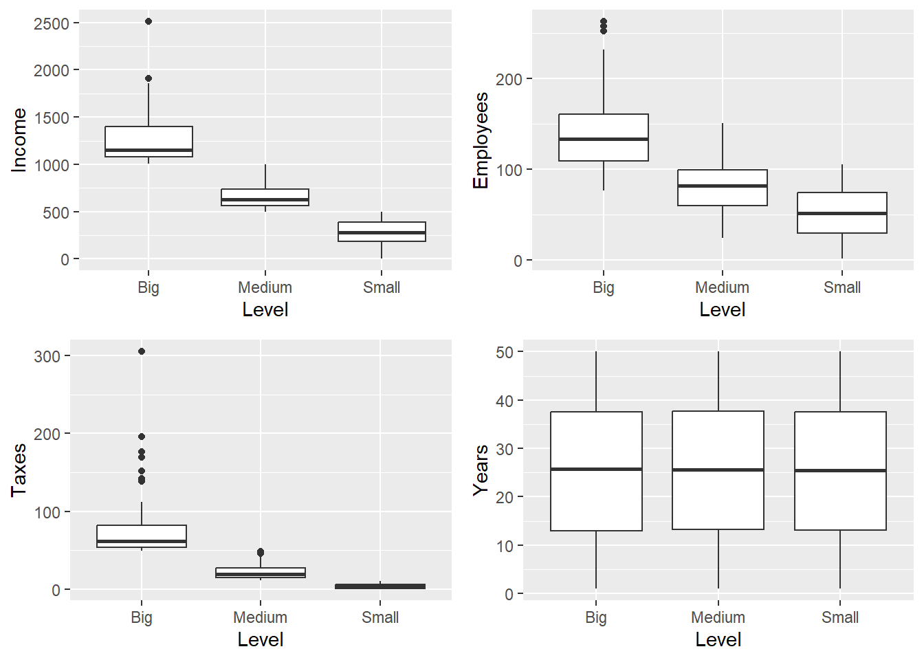
Of course, the government has created a policy plan with the promise of benefiting the electorate. If the government corroborates, through the present study, the hypothesis that SPAM influences the growth of some level of the industrial sector, then it will seek training and financing plans so that firms at the Medium and Small levels grow, stabilize, and promote the creation of new jobs and tax payments to the relevant government entities, and so that firms at the Large level do not move down a level but instead expand not only nationally but also internationally, where SPAM advertising can also arrive in a matter of microseconds.
For this new study, the government has provided a sampling frame that, in addition to containing the location and identification of all firms at all industrial levels, also includes the type of firm, namely: Large, Medium, Small. The type of firm will be taken as the stratification variable for the sampling plan design.
5.2.7.1 Estimation of sample size
The government is determined to implement a training plan for firms in the industrial sector and has requested that the sampling design be representative of the population with respect to the stratification characteristic: Level. For sample selection, the sampling frame must be loaded into the R environment. With the stratification variable Level, the sizes of each stratum are determined and must be converted into a vector of size \(H=3\), as in N <- c(N1,N2,N3); the same must be done with the sample sizes in each stratum, which must be converted into a vector as n <- c(n1,n2,n3).
data(BigLucy)
attach(BigLucy)

N1 <- summary(Level)[[1]]
N2 <- summary(Level)[[2]]
N3 <- summary(Level)[[3]]
N <- c(N1, N2, N3)
N
[1] 2905 25795 56596n1 <- round(2000 * N1 / sum(N))
n2 <- round(2000 * N2 / sum(N))
n3 <- round(2000 * N3 / sum(N))
n <- c(n1, n2, n3)
n[1] 68 605 1327Taking into account that proportional allocation is planned for estimating the sample size and that \(n=2000\) surveys are required, we have \(f=\frac{2000}{85296}=0.02345\). This implies carrying out \(n_1=\) 68 surveys of large firms, \(n_2=\) 605 surveys of medium firms, and \(n_3=\) 1327 surveys of small firms.
Using the S.STSI function from the TeachingSampling package, it is possible to select a simple random sample in each of the three strata. This function has three arguments. The first, Estrato, is the stratification variable indicating the membership of each and every one of the \(\sum_{h=1}^HN_h=N\) individuals in the population. The second argument, N, is a vector of size \(H\) indicating the sizes of each stratum in the population. The last argument, n, is a vector of size \(H\) indicating the sample sizes in each stratum. The result of the function is a set of indices that, when applied to the population, allows the stratified sample to be obtained.
sam <- S.STSI(BigLucy$Level, N, n)
sample_data <- BigLucy[sam, ]
head(sample_data)
ID Ubication Level Zone Income Employees Taxes SPAM ISO
34 AB0000000034 C0215234K0086663 Small County1 350 80 5 no no
65 AB0000000065 C0242828K0059069 Small County1 360 61 5 no no
153 AB0000000153 C0229084K0072813 Small County1 310 74 4 no no
360 AB0000000360 C0285599K0016298 Small County1 218 54 2 no no
406 AB0000000406 C0299340K0002557 Small County1 304 26 4 yes no
500 AB0000000500 C0121036K0180861 Small County1 296 45 3 yes no
Years Segments
34 46.0 County1 4
65 26.1 County1 7
153 22.0 County1 16
360 4.6 County1 36
406 2.8 County1 41
500 42.8 County1 50The realized (selected) sample has size 400 and is divided among the three strata. Once the selection of the elements has been carried out, information must be obtained through a survey of each firm in the industrial sector. Note that at this point, carrying out stratified sampling has logistical advantages. This is evident when it is decided that the questionnaire will be sent by email to each of the 14 firms at the Large level. Therefore, conducting this interview has enormous financial advantages because sending an email does not entail major expense. For the survey at the Medium level, it has been decided to hire a postal service agency and, in this way, send the questionnaire with the corresponding survey by certified mail. The same logistical means used for large firms is not applied because it is known that not all medium firms have an up-to-date email address, which does not happen in the large stratum. To obtain information from the industrial sector, trained interviewers have been sent to do the work. This is done because the owners of small firms are reluctant to answer certified letters and even less likely to answer email, since they have operational commitments to attend to.
Once the information from each of the 400 selected firms has been obtained, the quantities of interest are estimated. For this, the E.STSI function from the TeachingSampling package is used. This function has four sample parameters, namely: Estrato, the stratification variable indicating the membership of each and every one of the \(\sum_{h=1}^Hn_h=n\) individuals selected in the sample; N and n, the vectors of the population and stratified sample sizes, respectively; and target_variables, containing the value of the characteristic(s) of interest for each selected element.
target_variables <- data.frame(
  Income = sample_data$Income,
  Employees = sample_data$Employees,
  Taxes = sample_data$Taxes
)
E.STSI(sample_data$Level, N, n, target_variables)
The E.STSI function returns the estimate of each characteristic of interest disaggregated by stratum and the grand total, as well as the estimated variance and the estimated coefficient of variation. Note that, in terms of income, it is estimated that the large stratum produces 10%, the medium stratum 47%, and the small stratum 43% of the net income of the industrial sector. A similar result is observed for the remaining characteristics of interest. Note that the estimated coefficients of variation in each stratum are, in some cases, high5; however, the coefficient of variation for the total is low.
The following table shows the particular results for this exercise. It can be seen that stratification yields good results, with coefficients of variation smaller than those that would be produced by a simple random sample. This is because the variables of interest present, on average, different behavior in each stratum.
| Big | Medium | Small | Population | |
|---|---|---|---|---|
| Estimation | 2905 | 25795 | 56596 | 85296 |
| Standard Error | 0 | 0 | 0 | 0 |
| CVE | 0 | 0 | 0 | 0 |
| DEFF | NaN | NaN | NaN | NaN |
Income characteristic for each stratum and for the population.
| Big | Medium | Small | Population | |
|---|---|---|---|---|
| Estimation | 3578148.3 | 17045677.09 | 15909063.1 | 36532888.50 |
| Standard Error | 88124.4 | 133993.43 | 188799.1 | 247720.10 |
| CVE | 2.5 | 0.79 | 1.2 | 0.68 |
| DEFF | 1.0 | 1.00 | 1.0 | 0.25 |
Employees characteristic for each stratum and for the population.
| Big | Medium | Small | Population | |
|---|---|---|---|---|
| Estimation | 387518.5 | 2074387.0 | 2863706.4 | 5325611.88 |
| Standard Error | 13284.3 | 28478.6 | 39025.0 | 50104.46 |
| CVE | 3.4 | 1.4 | 1.4 | 0.94 |
| DEFF | 1.0 | 1.0 | 1.0 | 0.66 |
Taxes characteristic for each stratum and for the population.
| Big | Medium | Small | Population | |
|---|---|---|---|---|
| Estimation | 210826.1 | 569664.4 | 218259.2 | 998749.8 |
| Standard Error | 13661.6 | 9748.9 | 4934.4 | 17493.7 |
| CVE | 6.5 | 1.7 | 2.3 | 1.8 |
| DEFF | 1.0 | 1.0 | 1.0 | 0.3 |
The Domains function contained in the TeachingSampling package is used to obtain the indicator variables \(z_{dk}\) for each domain; the function’s only argument is a membership vector for each individual. In this case, the membership vector is SPAM. The output of this function is a matrix of ones and zeros, where each column is dichotomized. There are as many columns as there are population subgroups, and in each column the number one implies the element’s membership in the domain and zero its non-membership.
domains <- Domains(sample_data$SPAM)
spam_yes <- domains[, 2] * target_variables
spam_no <- domains[, 1] * target_variables

E.STSI(sample_data$Level, N, n, domains)
To estimate the absolute size of each domain, all that must be done is to multiply the matrix of characteristics of interest (in this case, the matrix called target_variables) by each column of the matrix resulting from dichotomization. Using the E.STSI function on the matrix resulting from dichotomization, we obtain the estimates of the absolute sizes of each domain. In this case, it is estimated that 1390 firms are already using other advertising techniques such as SPAM, while the remaining 1006 are not. In addition, in each of the three strata there are more firms using SPAM than not using it, and it is interesting that in the stratum of small firms, for every 2 firms that do not use SPAM there are 3 that do. Note that the variance of each estimate remains the same, because the values of this characteristic of interest are zeros and ones and, therefore, the variance structure is identical in each case.
| Big | Medium | Small | Population | |
|---|---|---|---|---|
| Estimation | 2905 | 25795 | 56596 | 85296 |
| Standard Error | 0 | 0 | 0 | 0 |
| CVE | 0 | 0 | 0 | 0 |
| DEFF | NaN | NaN | NaN | NaN |
spam_no domain for each stratum and for the entire population.
| Big | Medium | Small | Population | |
|---|---|---|---|---|
| Estimation | 684 | 9934.3 | 21324.8 | 31942.6 |
| Standard Error | 149 | 504.7 | 744.3 | 911.5 |
| CVE | 22 | 5.1 | 3.5 | 2.8 |
| DEFF | 1 | 1.0 | 1.0 | 1.0 |
spam_yes domain for each stratum and for the entire population.
| Big | Medium | Small | Population | |
|---|---|---|---|---|
| Estimation | 2221.5 | 15860.7 | 35271.2 | 53353.4 |
| Standard Error | 148.8 | 504.7 | 744.3 | 911.5 |
| CVE | 6.7 | 3.2 | 2.1 | 1.7 |
| DEFF | 1.0 | 1.0 | 1.0 | 1.0 |
It is clear that there is a trend in the industrial sector toward virtual advertising through email SPAM. The following figures are truly important because they show that firms in each of the three strata that use SPAM have higher income, employ more people, and contribute a larger amount of money in taxes; this occurs because there are more firms using SPAM than not using it. It should be kept in mind that within the subgroups (strata and domains), the coefficient of variation is high partly because of the disaggregation and partly because of the variance of the new variables.
Through the following computational code, the appropriate estimates are obtained for estimating the totals of the characteristics of interest in the spam_no domain. table 5.8, table 5.9, and table 5.10 show the point estimates for the selected sample.
E.STSI(sample_data$Level, N, n, spam_no)Income characteristic for the spam_no domain in each stratum and for the entire population.
| Big | Medium | Small | Population | |
|---|---|---|---|---|
| Estimation | 861503 | 6570050.5 | 5985144 | 13416698.12 |
| Standard Error | 190470 | 343776.0 | 239234 | 460101.86 |
| CVE | 22 | 5.2 | 4 | 3.43 |
| DEFF | 1 | 1.0 | 1 | 0.92 |
Employees characteristic for the spam_no domain in each stratum and for the entire population.
| Big | Medium | Small | Population | |
|---|---|---|---|---|
| Estimation | 87065 | 808172.3 | 1108377.4 | 2003614.26 |
| Standard Error | 19681 | 45447.9 | 45343.5 | 67148.15 |
| CVE | 23 | 5.6 | 4.1 | 3.35 |
| DEFF | 1 | 1.0 | 1.0 | 0.98 |
Taxes characteristic for the spam_no domain in each stratum and for the entire population.
| Big | Medium | Small | Population | |
|---|---|---|---|---|
| Estimation | 49684 | 220088.9 | 82526.9 | 352299.90 |
| Standard Error | 11355 | 12677.9 | 4222.4 | 17535.32 |
| CVE | 23 | 5.8 | 5.1 | 4.98 |
| DEFF | 1 | 1.0 | 1.0 | 0.85 |
On the other hand, using the following instruction, the appropriate estimates are obtained for estimating the totals of the characteristics of interest in the spam_yes domain. table 5.11, table 5.12, and table 5.13 show the point estimates for the selected sample.
E.STSI(sample_data$Level, N, n, spam_yes)Income characteristic for the spam_yes domain in each stratum and for the entire population.
| Big | Medium | Small | Population | |
|---|---|---|---|---|
| Estimation | 2716644.9 | 10475626.6 | 9923918.8 | 23116190.37 |
| Standard Error | 199285.0 | 349751.0 | 256706.8 | 477429.21 |
| CVE | 7.3 | 3.3 | 2.6 | 2.07 |
| DEFF | 1.0 | 1.0 | 1.0 | 0.71 |
Employees characteristic for the spam_yes domain in each stratum and for the entire population.
| Big | Medium | Small | Population | |
|---|---|---|---|---|
| Estimation | 300453.9 | 1266214.7 | 1755329.0 | 3321997.62 |
| Standard Error | 23488.9 | 45326.8 | 48297.0 | 70276.97 |
| CVE | 7.8 | 3.6 | 2.8 | 2.12 |
| DEFF | 1.0 | 1.0 | 1.0 | 0.87 |
Taxes characteristic for the spam_yes domain in each stratum and for the entire population.
| Big | Medium | Small | Population | |
|---|---|---|---|---|
| Estimation | 161142 | 349575.5 | 135732.3 | 646449.91 |
| Standard Error | 17062 | 13531.3 | 4797.9 | 22298.47 |
| CVE | 11 | 3.9 | 3.5 | 3.45 |
| DEFF | 1 | 1.0 | 1.0 | 0.57 |
Note that the value of the coefficients of variation is high because this is estimation in population subgroups where the sample size is random. In summary, the results show that the use of SPAM can be a growth strategy in the industrial sector. Now, thinking a little about the efficiency of the sampling strategy, consider the following analysis of variance table to calculate the design effect using Result 5.2.19.
anovaIL <- anova(lm(Income ~ Level, data = BigLucy))
anovaIL
Analysis of Variance Table
Response: Income
Df Sum Sq Mean Sq F value Pr(>F)
Level 2 4573694092 2286847046 133937 <0.0000000000000002 ***
Residuals 85293 1456301886 17074
---
Signif. codes: 0 '***' 0.001 '**' 0.01 '*' 0.05 '.' 0.1 ' ' 1The design effect would be given by dividing the residual variance by the variance of the variable; that is, \(\frac{17074.11}{70695.77}\) = 0.24. Therefore, the efficiency of the strategy is four times greater than that of a simple strategy. It is interesting that a design as simple as simple sampling in each stratum, with a small sample size, yields such good results.
Note that because \(N_d\) is unknown, to obtain another type of estimate (although not the variance or the estimated coefficient of variation) of the mean of the characteristic of interest in each domain, we can use an alternative estimator given by \[ \widehat{y}_{S_d}=\frac{\hat{t}_{yd,\pi}}{\hat{N}_{d,\pi}}=\frac{\sum_Sy_{dk}}{z_{dk}}=\frac{\sum_{S_d}y_k}{n_d} \]
To do this, we simply take the estimates \(t_{yd}\) and divide them by the estimate of \(N_d\).
5.2.7.2 Another type of allocation
Suppose that the government wants to conduct a survey with the characteristics and magnitudes of the previous one, but with an important limitation: money. The government has a budget of 7000 dollars for carrying out the study. In addition, the government wants the method used to collect the information to be classic. That is, an interviewer must go to each firm and administer the questionnaire. This case is very common in marketing surveys, where the goal is to obtain good estimates but there are not many financial or logistical resources available.
In this case, it has been found that the variances of the income variable are 64398, 16081, and 15142 in the Large, Medium, and Small strata, respectively. In addition, conducting a single survey in the stratum of large firms costs about 40 dollars, a survey in the stratum of medium firms costs 20 dollars, and an interview in the stratum of small firms costs 15 dollars. Note the price difference in each stratum; this is because high-profile interviewers must be hired for interviews in the stratum of large firms.
| Stratum | Cost | Nh | S2yuh | nh |
|---|---|---|---|---|
| Large | 40 | 83 | 64398 | 18 |
| Medium | 20 | 737 | 16081 | 112 |
| Small | 15 | 1576 | 15142 | 269 |
Using optimal allocation and Result 5.2.8, the sample sizes in each stratum, given by the previous table, minimize the variance of the Horvitz-Thompson estimator with the restriction of the study’s total cost, 7000 dollars. Note that \(\sum_{h=1}^3n_hC_h=7000\).
5.3 Stratified PPS sampling design
As seen in the previous section, the precision gain from using a stratified sampling design is important. However, the results can be improved by using a continuous auxiliary characteristic \(x_k\) that is well related to the characteristic of interest \(y_k\) in each stratum. Thus, it is possible to estimate the parameter of interest using the Hansen-Hurwitz estimator with a small variance. In fact, the stronger the correlation between \(y\) and \(x\), assuming that the average behavior of the variable of interest differs in each stratum, the smaller the variance of the Hansen-Hurwitz estimator.
In this case, the sampling frame must have two auxiliary characteristics: a stratification variable and continuous auxiliary information, both available for every element in all strata. It is assumed that the sampling design within each stratum is with replacement, and in this way a sample of size \(m_h\) is selected in each stratum \(h\) (\(h=1,\ldots,H\)). Each element \(k\in U_h\) has selection probability equal to \[ p_k = \dfrac{x_k}{t_{xh}} \ \ \ \text{if $k\in U_h$} \tag{5.4}\]
with \(t_{xh}\) the population total of the auxiliary characteristic \(x\) in stratum \(U_h\). It is important to verify that in each stratum \[ \sum_{U_h}p_k = 1\ \ \ \text{for each $h = 1,\ldots,H$}, \]
therefore \[ \sum_{h=1}^H\sum_{U_h}p_k = H \]
Now, in each stratum \(U_h\) of size \(N_h\), a sample \(s_h\) with replacement of size \(m_h\) is selected; therefore, the cardinality of the support in stratum \(U_h\) is given by \[ \#Q_h=\binom{N_h+m_h-1}{m_h} \]
The general stratified support is defined as the union of the supports in each of the strata \(U_h\). \[ Q^H=\left\{\bigcup_{h=1}^Hs_h\ \ \ \left|\right. \ \ s_h\in Q_h\right\}. \]
5.3.1 Selection algorithms
When selecting PPS samples with replacement in each stratum, it is possible to use the sampling algorithms given in Chapter 3, so the following steps must be carried out: - Separate the population into \(H\) strata using the stratification variable. - In each stratum \(U_h\), select a PPS sample with replacement. The algorithms used to select the sample within each stratum may be the total cumulative method or Lahiri’s method. - Each of the H selections is carried out independently.
5.3.2 The Hansen-Hurwitz estimator
Under the preceding conditions, the Hansen-Hurwitz estimator is used to unbiasedly estimate the parameter of interest \(t_y\) with the help of continuous auxiliary information in each stratum \(U_h\).
TipResult
If the elements within stratum \(U_h\) are selected with replacement according to selection probabilities such that \(\sum_{U_h}p_k = 1\), based on \(x_k\), the value of a continuous auxiliary characteristic, then the Hansen-Hurwitz estimator of the population total \(t_{yh}\), its variance, and its estimated variance are given by:
\[ \hat{t}_{yh,p}=\frac{t_{xh}}{m_h}\sum_{\substack{i=1\\k\in S_h}}^{m_h}\frac{y_{ki}}{x_{ki}} \] \[ Var_{PPS}(\hat{t}_{yh,p})=\frac{1}{m_h}\sum_{U_h}p_k\left(\frac{y_k}{p_k}-t_{yh}\right)^2 \] \[ \widehat{Var}_{PPS}(\hat{t}_{yh,p})=\frac{1}{m_h(m_h-1)}\sum_{\substack{i=1\\k\in S_h}}^{m_h}\left(\frac{y_{ki}}{p_{ki}}-\hat{t}_{yh,p}\right)^2 \] respectively, with \(p_k\) given by (equation 5.4). Note that \(\hat{t}_{yh,p}\) is unbiased for the total \(t_{yh}\) of the characteristic of interest \(y\), and that \(\widehat{Var}_{PPS}(\hat{t}_{yh,p})\) is unbiased for \(Var_{PPS}(\hat{t}_{yh,p})\).
TipResult
For a stratified sampling design with PPS selection of units in each stratum, the Hansen-Hurwitz estimator of the population total \(t_{y}\), its variance, and its estimated variance are given by:
\[ \hat{t}_{yh,p}=\sum_{h=1}^H\frac{t_{xh}}{m_h}\sum_{\substack{i=1\\k\in S_h}}^{m_h}\frac{y_{ki}}{x_{ki}} \] \[ Var_{STPPS}(\hat{t}_{yh,p})=\sum_{h=1}^H\frac{1}{m_h}\sum_{U_h}p_k\left(\frac{y_k}{p_k}-t_{yh}\right)^2 \] \[ \widehat{Var}_{STPPS}(\hat{t}_{yh,p})=\sum_{h=1}^H\frac{1}{m_h(m_h-1)}\sum_{\substack{i=1\\k\in S_h}}^{m_h}\left(\frac{y_{ki}}{p_{ki}}-\hat{t}_{yh,p}\right)^2 \] respectively. Note that \(\hat{t}_{y,p}\) is unbiased for the total \(t_{y}\) of the characteristic of interest \(y\), and that \(\widehat{Var}_{STPPS}(\hat{t}_{y,p})\) is unbiased for \(Var_{STPPS}(\hat{t}_{y,p})\).
NoteExample
For our example population \(U\), partitioned into 2 strata as in the previous chapter, there are, on the one hand, \(\binom{N_1+m_1-1}{m_1}=6\) possible samples with replacement of size \(m_1=2\) in the first stratum and, on the other hand, \(\binom{N_2+m_2-1}{m_2}=2\) possible samples with replacement of size \(m_2=1\) in the second stratum. Using the auxiliary characteristic \(x\), carry out the lexical-graphic calculation of the Hansen-Hurwitz estimator and verify unbiasedness and the variance.
5.3.3 Marco and Lucy
In the previous section, we assumed that the sampling frame contained, in addition to the location and identification of all firms in the industrial sector, a stratification variable called Level that groups firms according to their industrial production capacity. It is logical to think that the average behavior of the characteristics of interest differs in each stratum. Thus, the results obtained are more precise than when carrying out a simple sampling plan, in addition to obtaining the estimates of the characteristics of interest nested within the strata.
On this occasion, the construction of the sampling frame has managed to include, in addition to the stratification variable Level, continuous auxiliary information; in particular, it is assumed that the value of income declared in the last fiscal year is known for each firm in the industrial sector.
qplot(Income, Taxes, data = BigLucy, color = Level)qplot(Income, Taxes, data = Lucy, color = Level)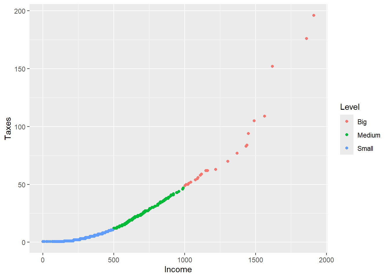
With this generous sampling frame, it is clear that the estimates will be more precise. However, it is worth asking whether the efficiency of the estimates will improve notably with these two auxiliary variables. Proportional allocation will be used, as in the previous section, to make the results comparable. Do not forget that in each stratum, sample selection is carried out with replacement.
data(BigLucy)
attach(BigLucy)

N1 <- summary(Level)[[1]]
N2 <- summary(Level)[[2]]
N3 <- summary(Level)[[3]]
N <- c(N1, N2, N3)
N
[1] 2905 25795 56596m1 <- round(2000 * N1 / sum(N))
m2 <- round(2000 * N2 / sum(N))
m3 <- round(2000 * N3 / sum(N))
m <- c(m1, m2, m3)
m[1] 68 605 1327The S.STPPS(E,x,m) function is used to draw the \(H\) samples with replacement in each stratum. The arguments of the function are the following: E, the stratification variable in the entire population, which in this particular case is Level; x, a vector of continuous auxiliary information containing each of the values in the population, which in this particular case is Income; and m, a vector containing \(H\) sample sizes for each stratum.
The S.STPPS(E,x,m) function divides the sampling frame into \(H\) strata and, in each one, selects a sample with replacement according to selection probabilities given by (5.3.1)6. The result of the function has two parts: on the one hand, the function returns the indices of the elements selected with replacement in each stratum and, on the other, it returns the vector of selection probabilities of the elements in the sample. Each of the preceding outputs has size \(m=\sum_{h=1}^Hm_h\). For this exercise, the result of the function has been saved in the object res, the sample in the object sam, and the vector of selection probabilities in the sample has been saved in the object pk.
res <- S.STPPS(BigLucy$Level, BigLucy$Income, m)
sam <- res[, 1]
pk <- res[, 2]
sample_data <- BigLucy[sam, ]
head(sample_data)
ID Ubication Level Zone Income Employees Taxes SPAM
11930 AB0000011930 C0188919K0112978 Big County26 1060 90 53 no
26322 AB0000026322 C0215358K0086539 Big County38 1450 162 94 yes
47904 AB0000047904 C0272968K0028929 Big County58 1551 168 107 no
19093 AB0000019093 C0069133K0232764 Big County31 1016 96 50 no
76653 AB0000076653 C0188155K0113742 Big County88 1008 76 50 no
4764 AB0000004764 C0147895K0154002 Big County19 1280 145 65 yes
ISO Years Segments
11930 yes 35.8 County26 12
26322 yes 48.4 County38 58
47904 yes 30.3 County58 15
19093 yes 40.0 County31 54
76653 yes 49.9 County88 20
4764 yes 4.1 County19 31By applying the indices obtained in sam to the sampling frame, we obtain the information needed to carry out the data collection process. When the information is collected, a data file will be created containing each of the values of the characteristic(s) of interest in the selected sample. This file is attached to R using the attach function.
The estimation stage is carried out with the E.STPPS(y,pk,m,E) function from the TeachingSampling package, whose four arguments each contain information at the sample level and only at the sample level: y, the data file containing each of the values of the characteristic(s) of interest in the selected sample, which in this particular case will be the data frame target_variables; pk, the vector of selection probabilities resulting from applying the S.STPPS function in the sample selection stage, saved in this particular case as pk <- res[,2]; m, a vector containing \(H\) sample sizes for each stratum, in this case given by m <- c(m1,m2,m3); and E, the stratification variable in the sample, in this particular case Level in the sample, not in the population.
The E.STPPS function returns the estimate of each characteristic of interest disaggregated by stratum and the grand total, as well as the estimated variance and the estimated coefficient of variation. It also returns the estimates of the stratum sizes \(\hat{N}_h\) and of the total population size given by \(\hat{N}=\sum_{h=1}^H\hat{N}_h\).
target_variables <- data.frame(
  Income = sample_data$Income,
  Employees = sample_data$Employees,
  Taxes = sample_data$Taxes
)
E.STPPS(target_variables, pk, m, sample_data$Level)| Big | Medium | Small | Population | |
|---|---|---|---|---|
| Estimation | 2926.2 | 25601.90 | 55014.3 | 83542 |
| Standard Error | 68.5 | 183.99 | 825.3 | 848 |
| CVE | 2.3 | 0.72 | 1.5 | 1 |
| DEFF | Inf | Inf | Inf | Inf |
Income characteristic for each stratum and for the population.
| Big | Medium | Small | Population | |
|---|---|---|---|---|
| Estimation | 3629710 | 17057285 | 15947738 | 36634733 |
| Standard Error | 0 | 0 | 0 | 0 |
| CVE | 0 | 0 | 0 | 0 |
| DEFF | 0 | 0 | 0 | 0 |
Employees characteristic for each stratum and for the population.
| Big | Medium | Small | Population | |
|---|---|---|---|---|
| Estimation | 408835.13 | 2079662.01 | 2862679.4 | 5351176.57 |
| Standard Error | 9240.70 | 25110.81 | 53263.6 | 59606.64 |
| CVE | 2.26 | 1.21 | 1.9 | 1.11 |
| DEFF | 0.29 | 0.85 | 2.0 | 0.94 |
Taxes characteristic for each stratum and for the population.
| Big | Medium | Small | Population | |
|---|---|---|---|---|
| Estimation | 222035.8 | 574362.39 | 221306.74 | 1017704.89 |
| Standard Error | 7830.3 | 4721.89 | 2398.93 | 9453.31 |
| CVE | 3.5 | 0.82 | 1.08 | 0.93 |
| DEFF | 0.2 | 0.24 | 0.25 | 0.07 |
Note that the estimates within the strata have a very small coefficient of variation, as does the estimate for the total population. The following table shows the results for this particular exercise.
| Variable | Population total | Estimated total | CVE % | Dev. % |
|---|---|---|---|---|
| Income | 1035217 | 1035217 | 0.00 | 0.00 |
| Employees | 151950 | 151570 | 0.07 | -0.25 |
| Taxes | 28654 | 28582 | 0.20 | -0.25 |
The efficiency gain of this sampling strategy is notable; there is not much more to say about it. One should simply exhaust all available resources to stratify the population and apply a PPS sampling design in each stratum, provided that the characteristic of interest is well correlated in each stratum with the auxiliary information.
5.4 Exercises
- Prove theoretically or refute by counterexample the following statements:
- To apply a stratified sampling design, the strata are required not to overlap. This condition is necessary to estimate the variance of the estimator.
- The need to stratify always arises from administrative reasons.
- A stratified sampling design always has lower variance than a sampling design that does not include strata.
- In a stratified sampling design, the estimate of the population average is the average of the estimates of the totals in each stratum.
- Explain a technical advantage of stratifying.
- Explain a logistical advantage of stratifying.
- Present in detail an example in which different sampling designs are proposed for different strata.
- Write the formulas for the total estimator and the variance estimator for the following sampling designs. Define each term and notation used in the formulas.
- Stratified design with three strata: one certainty inclusion stratum, one with a PPS design, and one with an SRS design.
- Stratified design with two strata: one certainty inclusion stratum and another with a systematic design.
- Stratified design with four strata: one certainty inclusion stratum, another with a Bernoulli design, another with an SRS design with replacement, and another with a Poisson design proportional to an auxiliary information characteristic.
- Stratified design with three strata: all with \(\pi\)PS design.
- Carry out the lexicographic exercise from Example 5.1.1.
- Carry out the lexicographic exercise from Example 5.2.2.
- Carry out the lexicographic exercise from Example 5.3.1.
- Suppose a population of four elements \(U=\{1,2,3,4\}\) whose values for the characteristic of interest are \(y_1=y_2=0\), \(y_3=1\), \(y_4=-1\). First, calculate the variance of the estimator of the population mean for a simple random sampling design with sample size \(n=2\). Then, calculate the variance of the estimator of the population mean for a sampling design with two strata \(U_1=\{1,2\}\) and \(U_2=\{3,4\}\) if a simple random design of size one is planned within each stratum. Which variance turned out to be larger? Explain.
- Suppose that a population of municipalities is divided into two strata, one urban and the other rural. Of all municipalities in the population, seven \((N_1=7)\) are cities and the remaining twenty-five \((N_2=25)\) are rural districts. It is decided that a stratified sampling design of total size \(n=8\) will be used. Taking the following table into account, determine sample sizes in each stratum according to proportional allocation, Neyman allocation, and optimal allocation.
| Rural stratum | Urban stratum | Total population | |
|---|---|---|---|
| Mean | 283 | 1146 | 472 |
| Std. dev. | 331 | 1318 | 743 |
| Size | 25 | 7 | 32 |
| Cost per survey | 5 pesos | 2 pesos | 3 pesos |
- Calculate the estimator of the population total, the estimator of the population mean, their respective estimated coefficients of variation, and confidence intervals for a sampling strategy that uses the Horvitz-Thompson estimator and a stratified random sampling design (\(H=2\)). The size of the first stratum is \(N_1=105\) and that of the second stratum is \(N_2=19\). For stratum one, a sample of \(n_1=11\) elements was selected, and for stratum two, a sample of \(n_2=4\) elements was selected. Use the following information:
| Stratum \(h\) | \(\sum_{s_h}y_k\) | \(\sum_{s_h}y_k^2\) |
|---|---|---|
| 1 | 1099 | 21855 |
| 2 | 3446 | 1822736 |
How to cite this book
Gutiérrez, A. (2027). Sampling strategies: Survey design and parameter estimation. Unpublished version online.
Fan, C., M. Muller, and I. Rezucha. 1962. “Development of Sampling Plans by Using Sequential (Item by Item) Selection Techniques and Digital Computer.” Journal of the American Statistical Association 57: 387–402.
Groves, R. M., F. J. Fowler, M. P. Couper, J. M. Lepkowski, E. Singer, and Tourangeau R. 2004. Survey Methodology. Wiley.
Lehtonen, R., and E. J. Pahkinen. 2003. Practial Methods for Design and Analysis of Complex Surveys. 2nd ed. New York: Wiley.
Lohr, S. 2000. Sampling: Design and Analysis. Thompson.
Sampath, S. 2001. Sampling Theory and Methods. Narosa Publishing House.
Valliant, R., A. H. Dorfman, and R. M. Royall. 2000. Finite Population Sampling and Inference. Wiley.
To divide the population into \(H\) disjoint strata.↩︎
This is due to independence among the selections. Even if it is known which units will be included in the sample of some stratum, this knowledge does not affect, in any way, the inclusion of any other unit in the remaining strata.↩︎
Note that \(S\) is a random variable and that the probability measures used to select samples in each stratum are different.↩︎
For example, in the presence of two sets \(A=\{a, b\}\) and \(B=\{1, 2\}\), the Cartesian product between \(A\) and \(B\) is \(A \times B = \{(a, 1), (a, 2), (b, 1), (b, 2) \}\).↩︎
The coefficient of variation is higher as estimates are more disaggregated into groups.↩︎
This function treats each stratum as a separate population so that the sum of the selection probabilities in each stratum is one and across the whole population sums to \(H\).↩︎