8 Estimation of Parameters Other than the Total

Naturally, the researcher is interested in finding the statistical properties of an estimator. If it has a linear form, no new tools are needed. However, the parameters encountered in practice correspond to nonlinear functions of totals.

Särndal et al. (1992)

In the preceding chapters, our attention focused on finding the best sampling design with Horvitz-Thompson estimators for sampling without replacement and Hansen-Hurwitz estimators for sampling with replacement. Along the way, we considered fixed and equal probability designs. To improve the efficiency of the strategy, we reviewed proportional-probability designs and stratified designs with the help of continuous or discrete auxiliary information. To improve the effectiveness of the operational plan and the dispersion of the sample across the population, complex cluster and multistage sampling designs were proposed.

The reader should have noticed that the first part of this text has faithfully followed the golden rule of survey design: use sampling strategies that induce inclusion or selection probabilities, as appropriate, proportional to the value of the characteristic of interest. Thus, if the survey focuses on a characteristic of interest with very low dispersion, such as the number of children in high socioeconomic groups, which is generally no greater than three, it is possible to use random sampling with simple probabilities. Otherwise, with the help of auxiliary information, the golden rule can be followed by constructing proportional probabilities at the design stage. However, this advantage of the sampling frame can be used not only at the design stage but also at the estimation stage.

8.1 Theoretical foundations

Following the philosophy reflected in the title of this text, we now continue the search for the best sampling strategy by improving the estimator. At this stage, the reader is assumed to know the structural behavior of the population and to be able to propose the best sampling design, according to how generous the sampling frame is.

Of course, in some multipurpose studies, complex surveys, and particular cases, estimates are needed for parameters other than totals. Examples include ratios of two characteristics of interest, population medians and percentiles, regression parameters, correlation coefficients, variances, covariances, indices, and so on. As Bautista (1998) states, the methodology proposed for estimating these population parameters is to rewrite them as functions of population totals. Thus, if the parameter to be estimated is \(B\), it should be written in the following form \[ B=f(t_1, t_2,\ldots,t_Q) \] where each \(t_q\), \(q=1,\ldots,Q\), represents a total of the characteristics of interest or a total of a function of the characteristics of interest. The estimation principle for this parameter is to obtain unbiased estimators \(\hat{t}_q\), \(q=1,\ldots,Q\), so that \(T\) is estimated by \[ \hat{B}=f(\hat{t}_1, \hat{t}_2,\ldots,\hat{t}_Q) \] Note that the function \(f\) may or may not be linear. A well-known result from classical statistical inference indicates that if \(f\) is a linear function, then \(B\) takes the form \[ B=a_0+\sum_{q=1}^Qa_qt_q \] Therefore, an unbiased estimator of \(B\) is given by the following expression \[ \hat{B}=a_0+\sum_{q=1}^Qa_q\hat{t}_q \] If Horvitz-Thompson-type estimators have been used to estimate \(B\), then (8.1.3) can be written as \[ \hat{B}_{\pi}=a_0+\sum_{k\in S}\frac{E_k}{\pi_k} \] where \(E_k=\sum_{q=1}^Qa_qy_{qk}\) and the value of the \(k\)-th element for the \(q\)-th characteristic of interest is given by \(y_{jk}\). Following the principles of the Horvitz-Thompson estimator, the variance of \(\hat{B}_{\pi}\) can be expressed as \[ Var(\hat{B}_{\pi})=\sum\sum_U\Delta_{kl}\frac{E_k}{\pi_k}\frac{E_l}{\pi_l}. \] An unbiased estimator for expression (8.0.5) is given by \[ \widehat{Var}_1(\hat{B}_{\pi})=\sum\sum_S \dfrac{\Delta_{kl}}{\pi_{kl}}\frac{E_k}{\pi_k}\frac{E_l}{\pi_l} \] Note that when the function \(f\) is linear, no new estimation principles are involved. By contrast, when \(f\) is nonlinear, the proposed estimator is still expression (8.1.2); however, in some cases, it is not possible either to compute or to estimate the variance because of the theoretical mathematical complexity of the derivation, and it becomes necessary to use methods that lead to an expression approximating the variance. The variance can be approximated using linearization techniques to estimate the precision of these estimators. These were introduced by Woodruff (1971). Applications in sampling theory have been developed, among others, by Binder (1983) and Deville (1999). The most common method, although not the only one, is Taylor polynomial linearization.

8.1.1 Approximation of a function by polynomials

Apostol (1963) (p. 417) presents the conditions under which a function \(f\) can be approximated by a polynomial. Among them are that the function \(f\) be differentiable and that its derivatives be defined at the point \(x=a\).

Taylor theorem

If a function can be approximated by a polynomial, then it is defined by \[ f(x)=f(a)+\frac{f'(a)}{1!}(x-a)+\frac{f''(a)}{2!}(x-a)^2+\ldots+\frac{f^{(n)}}{n!}(x-a)^n+\ldots \] Proof.

Let \[ f(x)=c_0+c_1(x-a)+c_2(x-a)^2+\ldots \] Differentiating successively, we have \[ \begin{aligned} &f^{(1)}(x)=c_1+2c_2(x-a)+3(x-a)^2+\ldots\\ &f^{(2)}(x)=2c_2+6c_3(x-a)+12c_4(x-a)^2+\ldots\\ &f^{(3)}(x)=6c_3+24c_4(x-a)+60c_5(x-a)^2+\ldots\\ \vdots\\ &f^{(n)}(x)=n!c_n+(n+1)!C_{n+1}(x-a)+(n+2)!C_{n+2}(x-a)^2+\ldots \end{aligned} \] Setting \(x=a\), we have \[ \begin{aligned} &f(a)=c_0 &f^{(1)}(a)=c_1\\ &f^{(2)}(a)=2c_2 &f^{(3)}(a)=6c_3 \end{aligned} \] and in general \(f^{(n)}(x)=n!c_n\). Substituting in (8.1.9) gives the Taylor polynomial approximation as in (8.1.8).

For vector-valued functions, the following Taylor theorem holds.

Result

For a vector-valued function \(f\), the first-order Taylor approximation of \(f\) at a (vector) point \(\mathbf{a}\) is given by \[ f(\mathbf{x})\cong f(\mathbf{a})+(\left.\nabla f\right|_{\mathbf{x}=\mathbf{a}})'(\mathbf{x}-\mathbf{a}), \] with \(\mathbf{x}=(x_1,\cdots,x_Q)'\), and \(\nabla f\) denotes the gradient of the function \(f\); that is, the \(q\)-th component of \(\nabla f\) is given by \[ \frac{\partial f(x_1,\cdots,x_Q)}{\partial x_q}. \]

Example

It is possible to represent the function \(\sin(x)\) as a power series in \(x\) (that is, at the point \(a=0\)). For this particular case, we have: \[ \begin{aligned} &f(x)=\sin(x) &f(0)=0&\\ &f^{(1)}(x)=\cos(x) &f^{(1)}(0)=1\\ &f^{(2)}(x)=-\sin(x) &f^{(2)}(0)=0\\ &f^{(3)}(x)=-\cos(x) &f^{(3)}(0)=-1\\ &f^{(4)}(x)=\sin(x) &f^{(4)}(0)=0\\ &\vdots &\vdots \end{aligned} \] Therefore, the series expansion of the function is as follows: \[ \begin{aligned} \sin(x)&=0+x+\frac{0}{2!}x^2+\frac{-1}{3!}x^3+\frac{0}{4!}x^4+\frac{1}{5!}x^5+\ldots\\ &=x+\frac{-1}{3!}x^3+\frac{1}{5!}x^5+\ldots\\\\ &=\sum_{n=1}^\infty \frac{(-1)^{n+1}}{(2n-1)!}x^{(2n-1)} \end{aligned} \] However, we must not only check whether the function and its derivatives are defined at a point \(x=a\); we must also check the convergence of the power series. For this, we use the ratio convergence test defined in Apostol (1963) (p. 363). This test states that if the value of \(R\), defined by \[ R=\lim_{n\rightarrow\infty}\left|\frac{S_{n+1}}{S_n}\right|, \] is less than one, then the series converges absolutely. For this particular example, we have \[ \begin{aligned} R&=\lim_{n\rightarrow\infty}\left|\frac{(-1)^{(n-1)+1}x^{2(n+1)-1}}{(2(n+1)-1)!}\Bigg/\frac{(-1)^{n-1}x^{2n-1}}{(2n-1)!}\right|\\ &=\lim_{n\rightarrow\infty}\left|\frac{x^{2n+1}}{(2n+1)!}\frac{(2n-1)!}{x^{2n-1}}\right|\\ &=x^2\lim_{n\rightarrow\infty}\left|\frac{1}{2n(2n+1)}\right|=0 \end{aligned} \] Therefore, the series converges absolutely, and we would have a good approximation to \(f(x)=sin(x)\) by truncating the series and leaving a negligible remainder.

8.1.1.1 Application in sampling

Using this technique, it is possible to approximate the variance of estimators that are not linear functions of totals. Although there is no unified asymptotic theory in finite-population inference, there are specific results for the simplest sampling designs (Madow 1948) and for some sampling designs with proportional probabilities (Rosén 1972). Lohr (2000) proposes the following steps to construct a linearized variance estimator for a nonlinear function of totals: - Express the estimator of the parameter of interest \(\hat{B}\) as a function of unbiased total estimators. Thus, \(\hat{B}=f(\hat{t}_1, \hat{t}_2,\ldots,\hat{t}_Q)\). - Determine all partial derivatives of \(f\) with respect to each estimated total \(\hat{t}_{q,\pi}\) and evaluate the result at the population quantities \(t_q\). Thus, \[ a_q=\left.\dfrac{\partial f(\hat{t}_1,\ldots,\hat{t}_Q)}{\partial \hat{t}_{q}}\right|_{\hat{t}_1=t_1,\ldots,\hat{t}_Q=t_Q} \] - Apply Taylor’s theorem for vector-valued functions to linearize the estimate \(\hat{B}\) with \(\mathbf{a}=(t_1,t_2,\cdots,t_Q)'\). In the previous step, we saw that \(\nabla\hat{B}'=(a_1,\cdots,a_Q)\). Consequently, \[ \hat{B}=f(\hat{t}_1,\ldots,\hat{t}_Q) \cong B+\sum_{q=1}^Qa_q(\hat{t}_{q}-t_q) \] - Define a new variable \(E_k\), with \(k\in S\), at the level of each element observed in the random sample. \[ E_k=\sum_{q=1}^Qa_qy_{qk} \tag{8.1}\] - From (8.1.12) and (8.1.13), if the estimators \(\hat{t}_{q}\) are Horvitz-Thompson estimators, an expression that approximates the variance of \(\hat{B}\) is given by \[ \begin{aligned} AVar(\hat{B})&=Var\left(\sum_{q=1}^Qa_q\hat{t}_{q,\pi}\right)\\ &=Var\left(\sum_S\frac{E_k}{\pi_k}\right)=\sum\sum_U\Delta_{kl}\frac{E_k}{\pi_k}\frac{E_l}{\pi_l}. \end{aligned} \] To find an estimate of the variance of \(\hat{B}\), it is not possible to use the values \(E_k\) directly, because they depend on the population totals: the derivatives \(a_q\) are evaluated at population totals that are unknown. Consequently, the values \(E_k\) are approximated by replacing the unknown totals with their estimators. Let \(e_k\) be the approximation of the linearized variable given by \[ e_k=\sum_{q=1}^Q\hat{a}_qy_{qk} \tag{8.2}\] where \(\hat{a}_q\) is an estimator of \(a_q\). On the other hand, Deville (1999) has shown that the variance approximation obtained through \(e_k\) is valid for large sample sizes. If the estimators \(\hat{t}_{q}\) are Horvitz-Thompson estimators, the Horvitz-Thompson variance estimator can generally be used, namely \[ \widehat{Var}(\hat{t}_{y,\pi})=\sum\sum_S \dfrac{\Delta_{kl}}{\pi_{kl}}\frac{e_k}{\pi_k}\frac{e_l}{\pi_l} \] As always, if the sampling design has fixed size, the corresponding expressions given in Chapter 2 of this text can be used. Särndal et al. (1992) warn that this method tends to underestimate the true variance when the sample size is small. Another disadvantage is that each approximation is specific to the functional form of the parameter of interest. Thus, particular analytical expressions must be determined, which becomes burdensome when working with complex surveys. The following result summarizes the general inference process for estimating a linearized function of totals.

Result

Let \(B=f(t_1, t_2,\ldots, t_Q)\) be a function of population totals. Then an approximately unbiased estimator of \(B\), its approximate variance, and an unbiased estimator of the latter are given by the following expressions \[ \begin{aligned} \hat{B}_{\pi} &= f(\hat{t}_{1,\pi}, \hat{t}_{2,\pi},\ldots,\hat{t}_{Q,\pi})\\ AVar(\hat{B}_\pi) &= \sum\sum_U\Delta_{kl}\frac{E_k}{\pi_k}\frac{E_l}{\pi_l}\\ \widehat{Var}(\hat{B}_\pi) &= \sum\sum_S \dfrac{\Delta_{kl}}{\pi_{kl}}\frac{e_k}{\pi_k}\frac{e_l}{\pi_l} \end{aligned} \] respectively, where \(\hat{t}_{q,\pi}\) is the Horvitz-Thompson estimator of \(t_{q,\pi}\) and both \(E_k\) and \(e_k\) are given by formulas (equation 8.1) and (equation 8.2), in that order.

Proof.

First, \[ \begin{aligned} E(\hat{B}_{\pi})&\cong E(B+\sum_{q=1}^Qa_q(\hat{t}_{q}-t_q))\\ &=B+\sum_{q=1}^Qa_qE(\hat{t}_{q}-t_q)\\ &=B \end{aligned} \] because \(\hat{t}_{q}\) is unbiased for \(t_q\), for \(q=1,\cdots,Q\). On the other hand, \[ \begin{aligned} Var(\hat{B}_\pi)&=Var(\sum_{q=1}^Qa_q\hat{t}_q)\\ &=Var(\sum_{q=1}^Qa_q\sum_{k\in S}\frac{y_{qk}}{\pi_k})\\ &=Var(\sum_{k\in S}\frac{E_k}{\pi_k})\\ &=\sum\sum_U\Delta_{kl}\frac{E_k}{\pi_k}\frac{E_l}{\pi_l} \end{aligned} \]

8.2 Estimation of a population ratio

A special case of a nonlinear function of totals is the population ratio \(B\). It is defined as the quotient of two population totals for characteristics of interest \(z\) and \(y\). Thus, \[ B=\dfrac{t_y}{t_z}=\dfrac{\bar{y}_U}{\bar{z}_U} \] Lohr (2000) notes that, technically, a ratio is always estimated when a domain mean is estimated. Note that a defining feature of the ratio is that both the denominator and the numerator are unknown, and even if they were known, it is preferable to estimate them. Bautista (1998) gives concrete examples in which ratio estimation has been used. Among them are the following: - Election studies: to estimate voting intention for a candidate, respondents are asked which candidate they would vote for¹. Since not all interviewed persons can vote, and some may even decide not to vote by omission, the numerator of this ratio is the total number of people who would vote for the candidate, while the denominator is the total number of people who would participate actively in the election. Note that the abstention rate is also given by a ratio. Its numerator would be the total number of people who, without any restriction, have decided not to participate in the election. Its denominator would be the total number of people eligible to vote. - Media research: television channels need an estimate of the total number of people watching a television program at a given time. With this information, channels charge more or less money to companies wishing to place an advertisement at a certain time. If the television program has a large audience, the channel will charge more for the advertisement slot. To standardize this information, an index called “rating” has been created; it is defined as the ratio between the total number of people watching a television program in a given minute and the total number of people watching television. - Social research: one of the economic indicators that attracts the most attention in the development of a region or country is the unemployment rate. It should be kept in mind that not all inhabitants of a region are able to work, since there is an age range for that. This economic indicator is defined as the population total of persons of working age who lack a job divided by the number of persons belonging to the economically active population.

For ratio estimation, the following result gives the theoretical expressions that should be used for this purpose.

Result

An estimator for the population ratio \(B\) of two characteristics of interest, its variance, and its estimated variance are given by \[ \begin{aligned} \hat{B} &= \dfrac{\hat{t}_{y,\pi}}{\hat{t}_{z,\pi}}\\ AVar(\hat{T}_{\pi}) &= \sum\sum_U\Delta_{kl}\frac{E_k}{\pi_k}\frac{E_l}{\pi_l}\\ \widehat{Var}(\hat{t}_{y,\pi}) &= \sum\sum_S \dfrac{\Delta_{kl}}{\pi_{kl}}\frac{e_k}{\pi_k}\frac{e_l}{\pi_l} \end{aligned} \] where \(E_k=\dfrac{1}{t_x}(y_k-Bz_k)\) and \(e_k=\dfrac{1}{\hat{t}_{z,\pi}}(y_k-\hat{B}z_k)\). Note that \(\hat{B}\) is approximately unbiased for \(B\), just as \(\widehat{Var}(\hat{t}_{y,\pi})\) is for \(AVar(\hat{t}_{y,\pi})\).

Proof.

Following the linearization steps from the previous section, the proposed estimator is a function of two estimated totals of the characteristics of interest: \[ \hat{B}=\dfrac{\hat{t}_{y,\pi}}{\hat{t}_{z,\pi}}=f(\hat{t}_{y,\pi},\hat{t}_{z,\pi}) \] Calculating the partial derivatives, \[ \begin{aligned} a_1&=\left.\dfrac{\partial f(\hat{t}_{y,\pi},\hat{t}_{z,\pi})}{\partial \hat{t}_{y,\pi}}\right|_{\hat{t}_{y,\pi}=t_y,\hat{t}_{z,\pi}=t_z}\\ &=\frac{1}{t_z}\\ a_2&=\left.\dfrac{\partial f(\hat{t}_{y,\pi},\hat{t}_{z,\pi})}{\partial \hat{t}_{z,\pi}}\right|_{\hat{t}_{y,\pi}=t_y,\hat{t}_{z,\pi}=t_z}\\ &=-\frac{t_y}{t_z^2} \end{aligned} \] Using the ratio approximation through expression (8.1.12), we have \[ \hat{B}=B+\frac{1}{t_z}(\hat{t}_{y,\pi}-t_y)-\frac{t_y}{t_z^2}(\hat{t}_{z,\pi}-t_z) \] therefore, when evaluating the expectation, the property of approximate unbiasedness follows immediately. On the other hand, defining the new linearized variable given in (8.1.14), we have \[ E_k=\dfrac{y_k}{t_z}-\frac{t_y}{t_z^2}z_k=\frac{1}{t_z}(y_k-Bz_k) \] whose approximation is \[ e_k=\frac{1}{\hat{t}_{z,\pi}}(y_k-\hat{B}z_k) \] Therefore, the variance is written as \[ AVar(\hat{B})=Var\left(\sum_S\frac{E_k}{\pi_k}\right) \] Using the principles of the Horvitz-Thompson estimator leads to the results for the variance approximation and the estimated variance.

It is not difficult to prove that, regardless of the sampling design used, the following conditions always hold: \[ \begin{aligned} \sum_UE_k&=0\\ \sum_S\frac{e_k}{\pi_k}&=0 \end{aligned} \] ### Properties

Although unbiasedness is a desirable property in estimators, it should not be taken so far as to discard estimators with a small amount of bias. In some cases, the functional form of the parameter of interest is so complex that obtaining an exactly unbiased estimator is very difficult. On the other hand, an estimator with little bias may have a smaller mean squared error than an unbiased estimator. In fact, Särndal et al. (1992) state that many approximately unbiased estimators are used in practice. They also state that one should always keep in mind Hájek’s rule, which proclaims that:

Estimators with considerable bias are poor, regardless of what other properties they may have.

Because this class of estimators is approximately unbiased, it is necessary to evaluate other desirable properties, such as the consistency given in the following definition.

Definition

An estimator \(\hat{T}\) is consistent in Cochran’s sense for a parameter of interest \(T\) if \(s=U\) implies that the estimator reproduces the parameter of interest. That is, \(\hat{T}=T\).

Note that under the class of SRS designs, the Horvitz-Thompson estimator is consistent because if \(s=U\), then \(\pi_k=1\); therefore, \[ \begin{aligned} \hat{t}_{y,\pi}=\sum_{k \in s}\frac{y_k}{\pi_k}=\sum_{k \in U}{y_k}=t_y \end{aligned} \] However, under the Bernoulli design, the Horvitz-Thompson estimator does not preserve consistency. Suppose that the first-order inclusion probabilities are given by \(\pi=0.1\). The event \(s=U\) occurs with probability \(0.1^N\), for which the Horvitz-Thompson estimator would take the following form: \[ \begin{aligned} \hat{t}_{y,\pi}=\sum_{k \in s}\frac{y_k}{0.1}=10\times t_y \end{aligned} \] Note that under this scenario, the ratio estimator \(\hat{B}\) is consistent.

8.2.1 Particular cases

The principles of the Horvitz-Thompson estimator are established in order to obtain an approximation and an estimate of the estimator’s variance. For the following sampling designs, the following properties hold.

8.2.1.1 Simple random sampling

For this particular sampling design, the first-order inclusion probabilities are given by \(\pi_k=\frac{n}{N}\). The Horvitz-Thompson estimators for the two characteristics of interest are given by \(\hat{t}_{y,\pi}=N\bar{y}_S\) and \(\hat{t}_{z,\pi}=N\bar{z}_S\). Therefore, the following result holds.

Result

Under simple random sampling, the estimator of the population ratio \(B\), its variance, and its estimated variance are given by \[ \begin{aligned} \hat{B} &= \dfrac{\bar{y}_S}{\bar{z}_S}\\ AVar_{SRS}(\hat{B}) &= \frac{N^2}{n}\left(1-\frac{n}{N}\right)S^2_{EU}\\ \widehat{Var}_{SRS}(\hat{B}) &= \frac{N^2}{n}\left(1-\frac{n}{N}\right)S^2_{es} \end{aligned} \] respectively, where \(S^2_{EU}\) and \(S^2_{es}\) are the variance estimator of the values of the linearized variable \(E\) and its approximation \(e\) in the universe \(U\) and in the sample \(s\). Recall that \(E_k=\dfrac{1}{t_x}(y_k-Bz_k)\) and \(e_k=\dfrac{1}{\hat{t}_{z,\pi}}(y_k-\hat{B}z_k)\).

8.2.1.2 Two-stage simple random sampling

For this sampling design, the Horvitz-Thompson estimators for the two characteristics of interest are given by \(\hat{t}_{y,\pi}=(N_I/n_I)\sum_{i\in S_I}N_i\bar{y}_{S_i}\) and \(\hat{t}_{z,\pi}=(N_I/n_I)\sum_{i\in S_I}N_i\bar{z}_{S_i}\). The following result holds.

Result

Under simple random sampling, the estimator of the population ratio \(B\), its variance, and its estimated variance are given by \[ \begin{aligned} \hat{B} &= \dfrac{\sum_{i\in S_I}N_i\bar{y}_{S_i}}{\sum_{i\in S_I}N_i\bar{z}_{S_i}}\\ AVar_{MS}(\hat{B}) &= \frac{N_{I}^2}{n_{I}}\left(1-\frac{n_{I}}{N_{I}}\right)S^2_{t_{E}U_I} + \frac{N_{I}}{n_{I}}\sum_{i\in U_{I}}\frac{N_i^2}{n_i}\left(1-\frac{n_i}{N_i}\right)S^2_{y_{E_i}}\\ \widehat{Var}_{MS}(\hat{B}) &= \frac{N_{I}^2}{n_{I}}\left(1-\frac{n_{I}}{N_{I}}\right)S^2_{\hat{t}_{e}S_I} + \frac{N_{I}}{n_{I}}\sum_{i\in S_{I}}\frac{N_i^2}{n_i}\left(1-\frac{n_i}{N_i}\right)S^2_{e_{S_i}} \end{aligned} \] respectively. Here, \(S^2_{t_{E}U_I}\) is the population variance of the totals \(t_{Ei}\), \(i\in U_I\), for each and every primary sampling unit, and \(S^2_{E_{U_i}}\) is the population variance among the values of the variable \(E\) taken by the elements within each primary sampling unit. The reasoning is similar for the quantities \(S^2_{\hat{t}_{e}s_I}\) and \(S^2_{y_{e_i}}\).

8.2.1.3 Sampling designs with proportional probability

Continuing with the golden rule of total estimation, both in strategies using sampling designs without replacement, such as Poisson or \(\pi\)PS, together with the Horvitz-Thompson estimator, and in sampling designs with replacement together with the Hansen-Hurwitz estimator, it was convenient for the sampling frame to include continuous auxiliary information in order to construct inclusion or selection probabilities, as appropriate.

Of course, in this particular context of ratio estimation, the sampling frame must be even more generous, to the extent that it allows the inclusion of continuous auxiliary information that should be correlated not with the characteristics of interest that enter the ratio but with the linearized variable \(E\). Thus, if the variable correlated with \(E\) is \(E^*\), then the optimal selection probabilities would be given by \[ p_k=\dfrac{E^*_k}{t_{E^*}} \] A similar argument applies to fixed-size designs that use proportional probabilities.

8.2.2 Estimation of a mean

One reason for using the estimator \(\hat{B}\) is that the population total \(N\) is unknown when estimating the population mean \(\bar{y}_U\). Even if \(N\) is known, it may be preferable to ignore it, as the following example shows (Lohr 2000). Suppose that, for some reason, an extraterrestrial wants to estimate the average number of legs that a dog has in a city. The city is divided into two geographic areas, the northern zone and the southern zone. To carry out the estimation, the extraterrestrial plans a two-stage sampling design as follows: from the \(N_I=2\) geographic zones of the city, a simple random sample of \(n_I=1\) primary sampling units will be selected. It is known that there are \(N_1=30\) dogs in the north and \(N_2=10\) dogs in the south. Whichever primary unit is selected, a simple random subsample of \(n_i=2\) dogs, \(i=1,2\), will be selected, and the total number of legs for each dog included in the sample will be measured.

Suppose that the northern zone has been selected. Curiously, in this zone each dog has the same number of legs, 4. The Horvitz-Thompson estimator of the total number of legs in the northern zone is \(\hat{t}_{1y,\pi}=\frac{30}{2}8=120\). Thus, an unbiased estimator of the total number of legs in the city is \(\hat{t}_{y,\pi}=\frac{2}{1}120=240\). Dividing this estimate by the total number of dogs in the city, we surprisingly find that the estimate of this mean is 6. \[ \hat{\bar{y}}_{U,\pi}=\frac{\hat{t}_{y,\pi}}{N}=\frac{240}{40}=6 \] Six legs! If the extraterrestrial’s sample had consisted of the southern zone, the Horvitz-Thompson estimator of the total number of legs in the southern zone would be \(\hat{t}_{2y,\pi}=\frac{10}{2}8=40\). The unbiased estimator of the total number of legs in the city would be \(\hat{t}_{y,\pi}=\frac{2}{1}40=80\). Dividing this estimate by the total number of dogs in the city, we find that the estimate of this mean is \[ \hat{\bar{y}}_{U,\pi}=\frac{\hat{t}_{y,\pi}}{N}=\frac{80}{40}=2 \] However, despite these results, the estimator is indeed unbiased because the expectation corresponds to the population parameter, since \((2+6)/2=4\). The extraterrestrial certainly did not use the best sampling strategy. This is not because of the choice of design, which induces constant inclusion probabilities as do the values of the characteristics of interest, but rather because of the choice of estimator. If the estimator used had been \(\hat{B}=\widetilde{y}_S\), defined in (2.2.15), the estimate would be \[ \widetilde{y}_S=\frac{\hat{t}_{y,\pi}}{\hat{N}}=\frac{240}{60}=4 \] when the northern zone is selected, because \(\hat{N}=\frac{2}{1}30=60\). Now, if the southern zone had been selected, we would have \(\hat{N}=\frac{2}{1}10=20\), and therefore \[ \widetilde{y}_S=\frac{\hat{t}_{y,\pi}}{\hat{N}}=\frac{80}{20}=4 \] Note that, for this particular case, the estimator \(\widetilde{y}_S\) is unbiased and has zero variance. The following result expands the properties of this estimator, which in the classical literature is called the weighted sample mean.

Result

An estimator of the population mean \(\bar{y}_U\), defined as a ratio, its variance, and its estimated variance are given by \[ \begin{aligned} \widetilde{y}_S &= \dfrac{\hat{t}_{y,\pi}}{\hat{N}_{\pi}}=\sum_S\dfrac{y_k}{\pi_k}\bigg/\sum_S\dfrac{1}{\pi_k}\\ AVar(\widetilde{y}_S) &= \frac{1}{N^2}\sum\sum_U\Delta_{kl}\left(\frac{y_k-\bar{y}_U}{\pi_k}\right)\left(\frac{y_l-\bar{y}_U}{\pi_l}\right)\\ \widehat{Var}(\widetilde{y}_S) &= \frac{1}{\hat{N}^2}\sum\sum_S \dfrac{\Delta_{kl}}{\pi_{kl}}\left(\frac{y_k-\widetilde{y}_S}{\pi_k}\right)\left(\frac{y_l-\widetilde{y}_S}{\pi_l}\right) \end{aligned} \] respectively.

This estimator coincides with the classical estimator \(\bar{y}_S\) in sampling designs such as simple random sampling or stratified random sampling.

8.2.2.1 Estimation of a mean in a domain

It is the rule, rather than the exception, that the absolute size \(N_d\) of a domain under study is unknown. Section 3.2.4 presented the basis for estimating the mean of the characteristic of interest in a domain when simple random sampling was used. This section provides the guidelines needed to carry out this estimation under any sampling design when \(N_d\) is unknown. Following the notation of Section 3.2.4, where the indicator function of the domain \(U_d\) given by (3.2.22) was defined and the variable \(y_{dk}\) was constructed, the following results are obtained for estimating \(N_d\) and for estimating the total of the characteristic of interest \(t_{yd}\) in the domain \(U_d\).

Result

Under any sampling design, the Horvitz-Thompson estimator for the absolute size of a domain \(N_d\), its variance, and its estimated variance are given by \[ \begin{aligned} \hat{N}_{d,\pi} &= \sum_S\frac{z_{dk}}{\pi_k}\\ Var(\hat{N}_{d,\pi}) &= \sum\sum_U\Delta_{kl}\frac{z_{dk}}{\pi_k}\frac{z_{dl}}{\pi_l}\\ \widehat{Var}(\hat{N}_{d,\pi}) &= \sum\sum_S \dfrac{\Delta_{kl}}{\pi_{kl}}\frac{z_{dk}}{\pi_k}\frac{z_{dl}}{\pi_l} \end{aligned} \] respectively.

Result

Under any sampling design, the Horvitz-Thompson estimator for the total of the characteristic of interest \(t_{yd}\) in the domain \(U_d\), its variance, and its estimated variance are given by \[ \begin{aligned} \hat{t}_{yd,\pi} &= \sum_S\frac{y_{dk}}{\pi_k}\\ Var(\hat{t}_{yd,\pi}) &= \sum\sum_U\Delta_{kl}\frac{y_{dk}}{\pi_k}\frac{y_{dl}}{\pi_l}\\ \widehat{Var}(\hat{t}_{yd,\pi}) &= \sum\sum_S \dfrac{\Delta_{kl}}{\pi_{kl}}\frac{y_{dk}}{\pi_k}\frac{y_{dl}}{\pi_l} \end{aligned} \] respectively.

Once the preceding parameters have been estimated, and following expression (3.2.23) for the mean of a domain, we proceed to estimate it using the following result.

Result

An estimator of the mean of a domain \(\bar{y}_{U_d}\), defined as a ratio, its variance, and its estimated variance are given by \[ \begin{aligned} \widetilde{y}_S &= \dfrac{\hat{t}_{y,\pi}}{\hat{N}_{\pi}}=\sum_S\dfrac{y_{dk}}{\pi_k}\bigg/\sum_S\dfrac{z_{dk}}{\pi_k}\\ AVar(\widetilde{y}_S) &= \frac{1}{N_d^2}\sum\sum_U\Delta_{kl}\left(\frac{y_{dk}-\bar{y}_{U_d}}{\pi_k}\right)\left(\frac{y_{dl}-\bar{y}_{U_d}}{\pi_l}\right)\\ \widehat{Var}(\widetilde{y}_S) &= \frac{1}{\hat{N}_d^2}\sum\sum_S \dfrac{\Delta_{kl}}{\pi_{kl}}\left(\frac{y_{dk}-\widetilde{y}_{S_d}}{\pi_k}\right)\left(\frac{y_l-\widetilde{y}_{S_d}}{\pi_l}\right) \end{aligned} \] respectively.

In the specific case of simple random sampling, the expression for the alternative estimator of the domain mean given by (3.2.26) coincides with the preceding results.

Example

Suppose that, for the example population \(U\), every value of the characteristics of interest x and y is known. Thus, the population ratio between the two is 0.7, as shown in the following output.

y <- c(32, 34, 46, 89, 35)
x <- c(52, 60, 75, 100, 50)
B <- sum(y) / sum(x)
B

[1] 0.7

With a simple random sample of \(n=2\), carry out the lexical-graphic calculation of the ratio estimator \(\hat{B}\). Repeat the exercise with a sample of \(n=4\) and, finally, with a complete enumeration or census. Conclude that this estimator is consistent.

8.2.3 Marco y Lucy

Continuing with the study of the industrial sector and based on the previous investigations, the government wants to estimate the ratio of total income in the industrial sector to the number of workers in that sector. This is a productivity index for the sector and describes how much revenue a single employee contributes to it. For the government, this index is important because it is used to build policies for distribution and financial support across the country’s economic sectors.

data(BigLucy)
ty <- sum(BigLucy$Income)
tz <- sum(BigLucy$Employees)
B <- ty / tz
B

[1] 6.8

In population terms, if we had carried out a census, this parameter would be equal to 6.79. In previous chapters, we learned how to draw samples and carry out the estimation process for the proposed strategies. In this chapter, we use the functions already established in the TeachingSampling package to compute the estimates and estimate the corresponding variances. Suppose that a simple random sampling design was used and that the selected sample is the one given in the corresponding Marco and Lucy section in the second chapter of this text. With the help of the S.SI and E.SI functions from the TeachingSampling package², the sample selection and total estimation are carried out, respectively. After selecting the sample, we proceed to estimate the population total with the relevant function. Recall that the output of the estimation function has the following form:

> E.SI(N,  n,  characteristic)
                      N                characteristic
Estimation            Position 1,1     Position 1,2
Standard Error        Position 2,1     Position 2,2
CVE                   Position 3,1     Position 3,2
DEFF                  Position 4,1     Position 4,2

Once the function parameters have been set, the values of the characteristic of interest are entered, and the function returns a matrix of estimates. In Position 1,2 we find the total estimate, in Position 2,2 we find the square root of the estimated variance, and in Position 3,2 we find the estimated coefficient of variation. To access each of these values independently, the function must be indexed; thus, if only the estimate of the population total for the income characteristic is desired, the following command must be written: E.SI(N,n,Income)[1, 2].

Here the index [1, 2] denotes the first element of the function. To estimate the ratio between the Income and Employees characteristics, we must estimate their respective totals with the help of the E.SI function and take the quotient between them.

N <- dim(BigLucy)[1]
n <- 2000
sam <- S.SI(N, n)
sample_data <- BigLucy[sam, ]

ty.est <- E.SI(N, n, sample_data$Income)[1, 2]
tz.est <- E.SI(N, n, sample_data$Employees)[1, 2]
B.est <- ty.est / tz.est
B.est

[1] 6.7

Although the estimate is available, we must estimate the variance approximation. For this purpose, we create the variables \(e_k\), \(k\in S\), and enter their values into the E.SI function to obtain the variance estimate. As mentioned earlier, this value of the variance estimate is indexed in the second position of the function.

ek <- (1 / tz.est) * (sample_data$Income - B.est * sample_data$Employees)
Asd <- E.SI(N, n, ek)[2, 2]
cve <- 100 * Asd / B.est
cve

[1] 1.1

The estimation result is presented in Table 8.1. Note that the estimated value is very close to the parameter of interest.

Table 8.1: Simple random sampling: estimation of the ratio of interest.

B	B.est	cve	Asd
6.8	6.7	1.1	0.07

Therefore, it is estimated that each employee contributed returns in the industrial sector of up to 6.92 million dollars in the last fiscal year. It would be interesting to know whether this ratio is constant for each level of the sector or whether there are differences in the ratio for each stratum. This topic will be addressed in the next chapter.

8.2.3.1 Central limit theorem

When considering the reliability and precision of the ratio estimator, the following question arises: can the central limit theorem be applied to ratio estimation?

Continuing with the empirical results, this section carries out a Monte Carlo simulation of size 2000 with the variables Income and Employees. For each simulation, a sample is selected and the corresponding ratio is estimated. The result of the simulation is a set of 2000 estimates displayed in histograms. The exercise was performed for sample sizes 2, 5, 20, 50, 200, and 1000. The graphical result of the simulation is shown in the following figure.

data(BigLucy)
N <- dim(BigLucy)[1]
nsim <- 2000
Bk <- rep(0, nsim)

Ratio <- function(n) {
  for (m in 1:nsim) {
    sam <- sample(N, n)
    x <- BigLucy$Income[sam]
    z <- BigLucy$Employees[sam]

    B <- mean(x) / mean(z)
    Bk[m] <- B
  }
  return(Bk)
}

simulations <- data.frame(
  Ratio(2), Ratio(5), Ratio(20),
  Ratio(50), Ratio(200), Ratio(1000)
)

p1 <- ggplot(data = simulations, aes(x = Ratio.2.)) +
  geom_histogram(aes(y = after_stat(density)), alpha = .5) +
  geom_density()
p2 <- ggplot(data = simulations, aes(x = Ratio.5.)) +
  geom_histogram(aes(y = after_stat(density)), alpha = .5) +
  geom_density()
p3 <- ggplot(data = simulations, aes(x = Ratio.20.)) +
  geom_histogram(aes(y = after_stat(density)), alpha = .5) +
  geom_density()
p4 <- ggplot(data = simulations, aes(x = Ratio.50.)) +
  geom_histogram(aes(y = after_stat(density)), alpha = .5) +
  geom_density()
p5 <- ggplot(data = simulations, aes(x = Ratio.200.)) +
  geom_histogram(aes(y = after_stat(density)), alpha = .5) +
  geom_density()
p6 <- ggplot(data = simulations, aes(x = Ratio.1000.)) +
  geom_histogram(aes(y = after_stat(density)), alpha = .5) +
  geom_density()
grid.arrange(p1, p2, p3, p4, p5, p6, ncol = 3)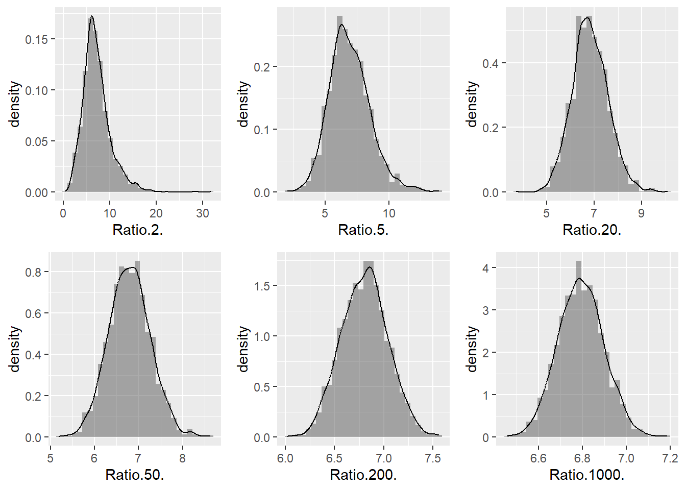

Figure 8.1: Sampling distribution of the estimated ratio.

For the first simulations, where the sample size is small, the ratio distribution is right-skewed; as the sample size grows, the distribution becomes symmetric around the true value. Thus, empirically and for this particular example, it has been shown that the ratio between these two characteristics converges to a normal distribution as the sample size increases.

8.3 Estimation of a median

A commonly used measure of central tendency is the median. Unlike the population mean, this measure of centrality is not easily influenced by outliers when the population size is small, and for this reason it is known as a robust measure. The median is the value \(M\) that divides the population into two halves. Therefore, half of the values of the characteristic of interest will be above \(M\) and the other half will be below \(M\). The construction of this and other estimates is based on the population distribution function \(F(\cdot)\).

Definition

For any value \(y\), the population distribution function \(F(y)\) is the proportion of elements in the population for which \(y_k\leq y\). This increasing function can be written as \[ F(y)=\dfrac{\#A_y}{N} \] con \(A_y\) dado por \[ A_y=\{ k \mid y_k\leq y, k\in U\} \]

From the previous definition, it is clear that any percentile³ \(Q_q\) with \(0 \leq q \leq 1\) can be written as a function of \(F(\cdot)\). Thus, \[ Q_q=F^{-1}(q) \] In particular, the median can be written as \(M=Q_{0.5}=F^{-1}(0.5)\). When a sampling design has been carried out and the selected sample information has been recorded, the generic procedure suggested in Särndal et al. (1992) (p. 197) for estimating any percentile consists of the following steps: - Obtain the estimated distribution function using the data for the characteristic of interest, \(\widehat{F}(y)\). - Estimate the percentile using \(\widehat{F}^{-1}(q)\). In particular, the median estimate would be given by \(\widehat{F}^{-1}(0.5)\).

As the following results indicate, no new estimation principles are involved in step 1 above. The procedure for estimating the distribution function can be viewed as estimating the population mean of the variable \(z_y\), which for the \(k\)-th element of the population is defined as \[ z_{yk}= \begin{cases} 1 &\text{if } y_k\leq y\\ 0 &\text{otherwise} \end{cases} \]

Result

The population distribution function can be written as a function of totals, specifically as a population mean, and is given by \[ \bar{z}_{yU}=\frac{t_{z_y}}{N}=\frac{1}{N}\sum_Uz_{yk}=F(y) \]

Result

An estimator of the population median \(M\) is given by \(\hat{M}\) \[ \hat{M}=\widehat{F}^{-1}(0.5), \] where \(\widehat{F}^{-1}\) is the inverse function of \(\widehat{F}(y)\), given by \[ \begin{aligned} \widehat{F}(e)&=\frac{\hat{t}_{z_y,\pi}}{\hat{N}}\\ &=\sum_S\frac{z_{yk}}{\pi_k}\left(\sum_S\frac{1}{\pi_k}\right)^{-1} \end{aligned} \]

This form of median estimation gives the same results as estimating a weighted median⁴ using the expansion factors given by \(1/\pi_k\), \(k\in S\). With this reasoning, we conclude that for sampling designs inducing equal inclusion probabilities for each element of the population, the median estimate corresponds to the median of the values of the characteristic of interest in the sample.

Therefore, if the values of the characteristic of interest in the realized sample are \(\{1,2,3\}\) and each element of that set is weighted by its corresponding expansion factor \(\{4,1,1\}\), then the estimated median coincides with the weighted median⁵, which is equal to the median of the following set \(\{\underbrace{1,1,1,1}_{4},\underbrace{2}_{1},\underbrace{3}_{1}\}\); that is, the median is one.

Example

For the example population \(U\), the population median is 35, as shown in the following output.

y <- c(32, 34, 46, 89, 35)
median(y)

[1] 35

If the vector of inclusion probabilities, induced by a design \(p(\cdot)\) with fixed sample size equal to \(n=4\), and the expansion factors are given by

pik <- c(1, 0.5, 1, 1, 0.5)
fk <- 1 / pik
fk

[1] 1 2 1 1 2

A possible sample belonging to the support \(Q\) of this sampling design is \[ s_1=\{\text{Yves, Ken, Erik, Sharon}\} \] Therefore, the median estimate for the data in this particular sample is 34, because

w <- c(32, 34, 34, 46, 89)
median(w)

[1] 34

How many possible samples have nonzero probability? Specify the support \(Q\) and, through a lexical-graphic calculation, conclude about the bias and consistency of the estimator \(\hat{M}\).

8.3.1 Marco y Lucy

In its effort to approach the central behavior of the characteristics of interest, the government planned the study from Section 4.2.4, where a PPS sampling design with selection probability proportional to size and sample size \(m=400\) was planned. On this occasion, knowledge of the characteristic of interest Income was used to create the selection probabilities of the elements. The results of the total estimates are truly close to the parameter of interest because of the strong correlation between the probabilities and the characteristics of interest.

However, the researchers associated with this project find that the structural behavior of the continuous auxiliary information Income is influenced by extreme points, as can be seen in the following figure. Moreover, it is known that the correlation between the characteristics of interest and the auxiliary information is high, and it is assumed that their structural behavior must also be highly dispersed. Therefore, as a measure of centrality, the decision has been made to work with the median because it is robust.

ggplot(BigLucy, aes(x = factor(0), y = Income)) +
  geom_boxplot() +
  xlab("") +
  coord_flip()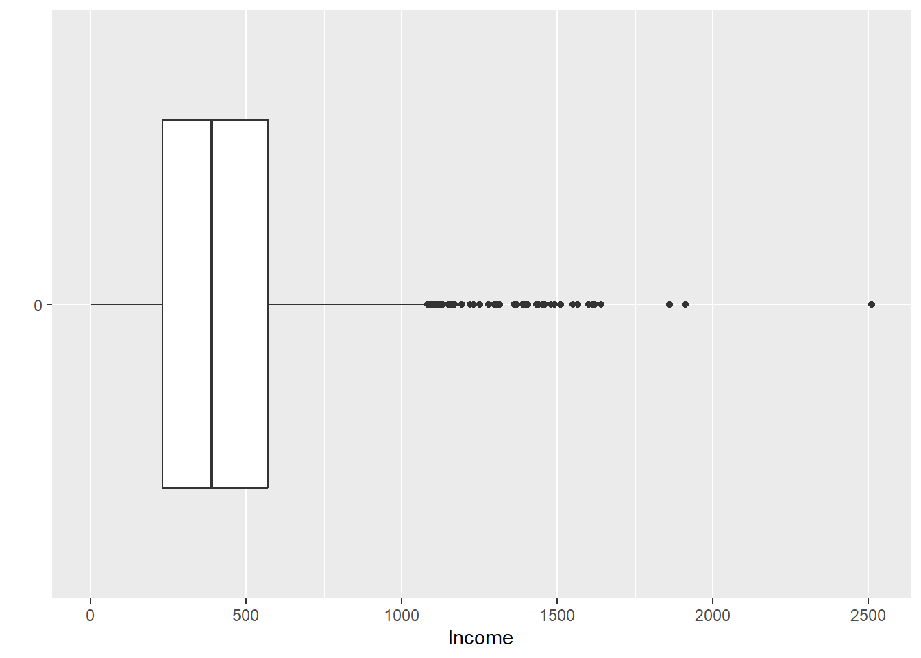

Figure 8.2: Dispersion of the continuous auxiliary information: `Income`.

Once the sample has been drawn, following the steps of Section 4.2.4 and with the help of the S.PPS and E.PPS functions, the E.Quantile function from the TeachingSampling package is used to estimate the median with the information collected in the sample.

data(BigLucy)
m <- 2000
res <- S.PPS(m, BigLucy$Income)
sam <- res[, 1]
sample_data <- BigLucy[sam, ]

The nature of this exercise is very interesting because it is a with-replacement design. Once the sample is selected, the vector of selection probabilities must be extracted for the firms selected in the sample. The E.Quantile function has three parameters: y, which, as usual, is the data set containing the information collected in the sample for the characteristic(s) of interest; per, which is the percentile of interest and takes values from 0 to 1, in this case 0.5, corresponding to the median; and finally pik, which contains the inclusion probabilities for each element selected in the sample⁶. If this argument is left empty, the function result will be the corresponding percentile for the values of y, treating the sample as if it were a population.

pk.s <- res[, 2]
pik <- 1 - (1 - pk.s)^m

target_variables <- data.frame(
  Income = sample_data$Income,
  Employees = sample_data$Employees,
  Taxes = sample_data$Taxes
)
E.Quantile(target_variables, 0.5, pik)

[1] 400  75  15

The function result gives the following estimates: - For the auxiliary information income in the last fiscal year, the estimated median is 420 million dollars. - For the characteristic of interest number of employees, the estimated median is 73. - For the characteristic of interest taxes declared in the last fiscal year, the estimated median is 12 million dollars.

If this sample had been analyzed without taking the sampling design into account, the estimates would be completely different and therefore incorrect.

8.4 Estimation of regression coefficients

We have reached the most important section, the one that gives this part its name: inference assisted by population models. Once we have laid out the theoretical and philosophical foundations that motivate a model in a finite population, we can improve many kinds of estimators for most parameters of interest. It is essential for the reader to review the information in this section repeatedly until achieving full understanding and genuine engagement with the topic. Once the reader fully understands the spirit of this section, they will be able not only to delve into more complex and interesting topics in sampling and finite-population inference, but also to begin rigorous research work to create, build, or improve the estimators proposed in the classical literature.

In finite-population inference based on the sampling design, emphasis is placed on the idea that the statistical properties of the strategy used to estimate the parameters of interest must be governed by the sampling design that has been used. Thus, in the previous chapters, the expectation, the variance calculation, and the variance estimation were carried out by assuming a sampling design \(p(\cdot)\) and by considering the values \(y_1,y_2\ldots, y_N\) that the characteristic of interest can take as fixed pseudo-parameters that are not subject to change.

When continuous or categorical auxiliary information is known in the sampling frame, we say that for each element in the population there is a vector of auxiliary information that takes the value \(\mathbf{x}_k\) for the \(k\)-th unit. If this vector contains \(p\) auxiliary characteristics, then it takes the following form: \(\mathbf{x}_k=(x_{1k}, x_{2k},\ldots,x_{pk})'\).

However, when the goal is to determine the relationship between the characteristic of interest and the continuous or categorical auxiliary information contained in the sampling frame, it is necessary to use a probabilistic model that requires another type of assumptions. Although these assumptions must be handled very carefully, they do not contradict the theory proposed so far.

8.4.1 Theoretical foundations

Suppose that there are \(N\) random variables \(Y_1,Y_2,\ldots,Y_N\), and that there is also a vector of random variables \(\mathbf{X}_1,\mathbf{X}_2,\ldots,\mathbf{X}_N\), with the relationship between these random variables given by a probability model \(\xi\)⁷ such that \[ Y_k=\mathbf{X}_k'\boldsymbol{\beta}+\varepsilon_k \] where each of the \(\varepsilon_k\), \(k\in U\), are independent and identically distributed random variables with mean zero and variance⁸ \(c_k\sigma^2\). The vector \(\boldsymbol{\beta}\) is known as the vector of regression coefficients in the superpopulation model, or the regression super-parameter. Under the variables \(\varepsilon_k\), the following properties hold.

Result

The expectation and variance of the random variables \(Y_k\) are given by \[ \begin{aligned} E_{\xi}(Y_k)&=\mathbf{X}_k'\boldsymbol{\beta} \\ Var_{\xi}(Y_k)&=c_k\sigma^2. \end{aligned} \tag{8.3}\] Proof.

The statistical properties concern the proposed model \(\xi\) and \(\varepsilon_k\), assuming that the auxiliary information is fixed. Thus, \[ \begin{aligned} E_{\xi}(Y_k)&=E_{\xi}\left(\mathbf{X}_k'\boldsymbol{\beta}+\varepsilon_k\right)\\ &=\mathbf{X}_k'\boldsymbol{\beta}+E_{\xi}(\varepsilon_k)\\ &=\mathbf{X}_k'\boldsymbol{\beta}. \end{aligned} \] On the other hand, we have \[ \begin{aligned} Var_{\xi}(Y_k)&=Var_{\xi}\left(\mathbf{X}_k'\boldsymbol{\beta}+\varepsilon_k\right)\\ &=Var_{\xi}(\varepsilon_k)\\ &=c_k\sigma^2. \end{aligned} \] Note that the subscript \(\xi\) denotes that inference is carried out under the distribution function induced by the model.

Under this superpopulation model, the values \(y_1,y_2,\ldots,y_N\) for the characteristic of interest are considered realizations of the random variables \(Y_1,Y_2,\ldots,Y_N\). The same is true for the values of the vector \(\mathbf{x}_1,\mathbf{x}_2,\ldots,\mathbf{x}_N\), which are considered realizations of the random vectors \(\mathbf{X}_1,\mathbf{X}_2,\ldots,\mathbf{X}_N\). The model \(\xi\) given by (8.4.1) and (8.4.2) is very general and allows all kinds of interpretations. But before entering into each possible model of interest, it is necessary to go a little deeper into its philosophical foundations.

Under the model \(\xi\), a relationship between random variables is assumed, given by the vector of regression coefficients \(\boldsymbol{\beta}\) and by the random variables \(\varepsilon_k\). Cassel et al. (1976) state that \(\xi\) is known as a superpopulation model because it assumes that the finite population \(U\) is treated as if it had been selected from an even larger universe containing all kinds of possible values for \(Y_k\) and \(\mathbf{X}_k\). Since it is impossible for us to calculate the value of \(\boldsymbol{\beta}\) because, in some sense, we are not conditioned to know the state of nature of the model in question, \(\boldsymbol{\beta}\) must be estimated using the finite-population data \(Y_1,Y_2,\ldots,Y_N\) and \(\mathbf{x}_1,\mathbf{x}_2,\ldots,\mathbf{x}_N\) by carrying out a census.

8.4.2 Estimation in the finite population

When the information collected in the census is available; that is, when the realizations given by \(y_k\) and \(\mathbf{x}_k\) (\(k\in U\)) are known, one way, though not the only one, to estimate the regression super-parameter \(\boldsymbol{\beta}\) is to use the least squares method, which yields an estimate \(\mathbf{B}\).

Within the range of possible values that the estimator \(B\) can take, the least squares method assigns to \(B\) the value that minimizes the following function: \[ D=\sum_U \left(\frac{y_k-\mathbf{x}_k'\mathbf{B}}{c_k\sigma^2}\right)^2. \] Once again, note that neither \(y_k\) nor \(\mathbf{x}_k\) are random variables; rather, they must be treated as realizations of random variables. Thus, the relationship is assumed to induce a vector of regression coefficients estimated in the finite population \(U\), which can be obtained by fitting the hyperplane \(y_k=B_1x_{1k}+\ldots+B_px_{pk}\) for the \(N\) elements in the entire population. The following result shows the form of the least squares estimator. To improve understanding of the results presented in this section, some expressions will be written in matrix language, so that the reader quickly becomes familiar with linear models.

Result

Using the least squares method, the estimator of \(\boldsymbol{\beta}\) in the finite population \(U\) is given by \[ \begin{aligned} \mathbf{B}=(B_1,\ldots,B_p)'&=\left(\mathbf{x}\Sigma^{-1}\mathbf{x}'\right)^{-1}\left(\mathbf{x}\Sigma^{-1}\mathbf{y}\right)\\ &=\left(\sum_U\dfrac{\mathbf{x}_k\mathbf{x}_k'}{c_k\sigma^2}\right)^{-1}\sum_U\dfrac{\mathbf{x}_ky_k}{c_k\sigma^2}\\ &=\left(\sum_U\dfrac{\mathbf{x}_k\mathbf{x}_k'}{c_k}\right)^{-1}\sum_U\dfrac{\mathbf{x}_ky_k}{c_k} \end{aligned} \] where \[ \mathbf{x}=\left( \begin{array}{ccc} x_{11} & \ldots & x_{1N} \\ \vdots & \ddots & \vdots \\ x_{p1} & \ldots & x_{pN} \\ \end{array} \right)=\left( \begin{array}{ccc} \mathbf{x}_1 & \ldots & \mathbf{x}_N \\ \end{array} \right); \ \ \ \ \ \ \ \mathbf{y}=\left( \begin{array}{c} y_1 \\ \vdots \\ y_N \\ \end{array} \right). \] and \(\Sigma\) is a diagonal matrix of size \(N\times N\) given by \[ \Sigma=\left( \begin{array}{ccc} c_1\sigma^2 & \ldots & 0 \\ \vdots & \ddots & \vdots \\ 0 & \ldots & c_N\sigma^2 \\ \end{array} \right) \] Proof.

The expression to be minimized is (8.4.3), which corresponds to the sum of squared errors \(\mathbf{E}=\mathbf{y}-\mathbf{x}'\mathbf{B}\) weighted by \(c_k\sigma^2\), and can be rewritten as follows: \[ \begin{aligned} D&=\mathbf{E}'\Sigma^{-1}\mathbf{E}\\ &=(\mathbf{y}-\mathbf{x}'\mathbf{B})'\Sigma^{-1}(\mathbf{y}-\mathbf{x}'\mathbf{B})\\ &=\mathbf{y}'\mathbf{y}-2\mathbf{B}'\mathbf{x}\Sigma^{-1}\mathbf{y}+\mathbf{B}'\mathbf{x}\Sigma^{-1}\mathbf{x}'\mathbf{B} \end{aligned} \] Differentiating with respect to \(\mathbf{B}\) and setting the result equal to zero, \[ \begin{aligned} \frac{\partial D}{\partial \mathbf{B}}=-2\mathbf{x}'\Sigma^{-1}\mathbf{y}+2\mathbf{x}'\Sigma^{-1}\mathbf{x}\mathbf{B}\equiv 0 \end{aligned} \] we obtain the proof of the result.

Although it is not the only method, the least squares technique stands out because of its estimation properties. The reader should likely be familiar with regression methods, although for the novice reader Ravishanker and Dey (2002) is recommended for a good understanding of linear model theory. Other approaches exist for estimating \(B\), such as local polynomial regression techniques (Breidt and Opsomer 2000) or robust nonparametric techniques (Gutiérrez 2009; Gutiérrez and Breidt 2009). It is essential for the reader to note that the theoretical foundation never made any assumption about the distribution function of the random variables \(\varepsilon_k\), and therefore the inference remains free of assumptions about theoretical distributions.

8.4.3 Estimation in the sample

Of course, in practice we do not have access to all values of the characteristic of interest; in many cases, we do not even have access to all values of the auxiliary information for each element in the finite population. Thus, the regression coefficient must be estimated. For this purpose, and following the guidelines of the introductory section, \(B\) is expressed as a function of totals. Indeed, we have: \[ \begin{aligned} \mathbf{B}&=\mathbf{T^{-1}t} \end{aligned} \] where \[ \begin{aligned} \mathbf{T}=\sum_U\dfrac{\mathbf{x}_k\mathbf{x}_k'}{c_k} \end{aligned} \] and \[ \begin{aligned} \mathbf{t}=\sum_U\dfrac{\mathbf{x}_ky_k}{c_k} \end{aligned} \]

Result

Using the principles for estimating a function of totals, when the least squares method is used, \(\mathbf{B}\) is estimated by \[ \hat{\mathbf{B}}=\hat{\mathbf{T}}^{-1}\hat{\mathbf{t}} \] where \[ \begin{aligned} \mathbf{T}=\sum_S\dfrac{\mathbf{x}_k\mathbf{x}_k'}{\pi_kc_k} \end{aligned} \] and \[ \begin{aligned} \mathbf{t}=\sum_S\dfrac{\mathbf{x}_ky_k}{\pi_kc_k} \end{aligned} \] Note that \(\hat{\mathbf{T}}\) and \(\hat{\mathbf{t}}\) are unbiased estimators for \(\mathbf{T}\) and \(\mathbf{t}\), respectively. However, \(\hat{\mathbf{B}}\) is not unbiased for \(\mathbf{B}\).

Although the estimator of \(\mathbf{B}\) is biased, an expression for the variance must be found. Särndal et al. (1992) show that when the Taylor linearization method is used, the variance approximation of estimator (8.4.12) is given by \[ AV(\mathbf{\hat{B}})=\left(\sum_U \frac{\mathbf{x}_k\mathbf{x}_k'}{\sigma^2_k}\right)^{-1}\mathbf{V}\left(\sum_U \frac{\mathbf{x}_k\mathbf{x}_k'}{\sigma^2_k}\right)^{-1}, \] where \(\mathbf{V}\) is a symmetric matrix of size \(p\times p\) whose entries are \[ v_{ij}=\sum\sum_U \Delta_{kl}\left(\frac{x_{ik}E_k}{\pi_k}\right)\left(\frac{x_{jl}E_l}{\pi_l}\right) \] and \(E_k=y_k-\mathbf{x}_k'\mathbf{B}\). The estimator of the variance approximation is \[ \widehat{Var}(\mathbf{\hat{B}})=\left(\sum_s \frac{\mathbf{x}_k\mathbf{x}_k'}{\sigma^2_k\pi_k}\right)^{-1}\hat{\mathbf{V}}\left(\sum_s \frac{\mathbf{x}_k\mathbf{x}_k'}{\sigma^2_k\pi_k}\right)^{-1}, \] where \(\mathbf{V}\) is a symmetric matrix of size \(p\times p\) whose entries are \[ \hat{v}_{ij}=\sum\sum_s \frac{\Delta_{kl}}{\pi_{kl}}\left(\frac{x_{ik}e_k}{\pi_k}\right)\left(\frac{x_{jl}e_l}{\pi_l}\right) \] and \(e_k=y_k-\mathbf{x}_k'\hat{\mathbf{B}}\). Note that \(i,j=1,\ldots,p\).

8.4.4 Special cases

The general linear model, defined by expressions (8.4.1) and (8.4.2), includes many special cases of potential practical interest for the user who wants to verify or estimate the relationship between the characteristic of interest and the auxiliary information. Note that this general model has no restriction on the nature of the auxiliary information. That is, the auxiliary information vector \(\mathbf{x}_k\) can be continuous or categorical.

There are three vitally important concepts related to the interpretation and fitting of any model in a finite population. They are: - Model level: specifies the sampling unit used in the formulation of the model. A model is said to be fitted at the element level when it is formulated in terms of auxiliary information available for all elements of the finite population \(U\). A model can be formulated both at the element level and at the cluster level. For multistage designs, many models can be formulated at different levels. - Model type: this concept refers to fitting the best model that explains the relationship between the characteristic of interest and the auxiliary information. How many variables should be included in the model? What variance structure should be proposed? Should the model have an intercept? - Group model: when it is known that the finite population \(U\) can be partitioned into population groups, it is possible to fit a general model that works well in the finite population. However, when it is known that this partition affects the structural behavior of the characteristic of interest in each group, it is advisable to fit a model in each group. Thus, if the population is composed of \(G\) groups, \(G\) models will be fitted, one for each group. Note that this partition may be defined either at the element level or at the population level.

Although the general linear model applies to many cases, it is the user’s responsibility to be able to propose the best model. As the master Bengt Swensson stated in an interview given in 2005:

[The general linear model] states that there is a relationship with the auxiliary information. To me, those are just data that do not carry information by themselves. However, they have the potential to do so. Whether the data are useful in estimation will depend on how \(\mathbf{x}\) is related to \(\mathbf{y}\). If the statistician’s knowledge and experience (based on previous surveys, pilot samples, or any other evidence) indicate that \(\mathbf{x}\) does indeed have a strong relationship with \(\mathbf{y}\), then the model begins to make sense. The more knowledge one has, the better the model that can be fitted.

Although many combinations exist, with respect to model type it is common to find the following models in the classical literature:

Common mean model: this model assumes that the characteristic of interest has the same common relationship for every element in the population and that the variance structure is constant. Thus \(p=1\), \(\mathbf{x}_k=1\), and \(c_k=1\) for all \(k\in U\). The model formulation is given by \[ Y_k=\beta+\varepsilon_k \] where each of the \(\varepsilon_k\), \(k\in U\), are independent and identically distributed random variables with mean zero and variance \(\sigma^2\).

N <- 500
b <- 10
sigma <- 2

z <- c(1:N)
x <- rep(1, N)
e <- rnorm(N, 0, sigma)
y <- b * x + e

data <- data.frame(x, y)
ggplot(data, aes(x = z, y = y)) +
  geom_point(shape = 1) +
  geom_smooth(method = "lm")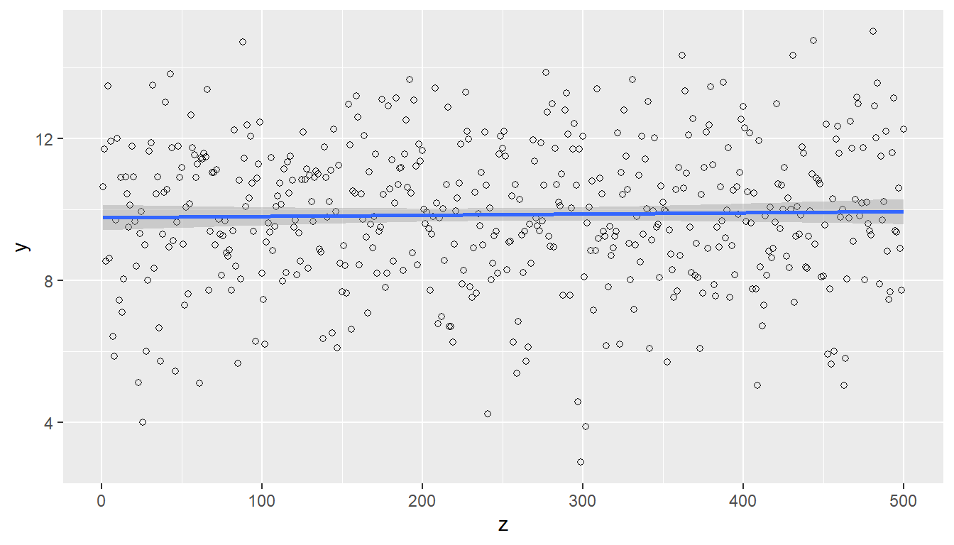

Figure 8.3: Scatterplot for a common mean model.

figure 8.3 shows the behavior of the relationship between the auxiliary information and the characteristic of interest. This model has the following properties: \[ \begin{aligned} E_{\xi}(Y_k)&=\beta \\ Var_{\xi}(Y_k)&=\sigma^2. \end{aligned} \] The sample-based estimator of the regression coefficient is given by \[ \hat{\mathbf{B}}=\left(\sum_S\frac{1}{\pi_k}\right)^{-1}\left(\sum_S\frac{y_k}{\pi_k}\right)=\frac{\hat{t}_{y,\pi}}{\hat{N}_{\pi}}=\widetilde{y}_S \] Thus, under this model, the alternative estimator of the mean, or weighted sample mean, is a special case of the regression coefficient.

Ratio model: this model assumes the existence of a single continuous auxiliary information variable related to the characteristic of interest and that the variance structure is inversely proportional to the structural behavior of the auxiliary information. Thus \(p=1\), \(\mathbf{x}_k=x_k\), and \(c_k=x_k\) for all \(k\in U\). The model formulation is given by \[ Y_k=X_k'\beta+\varepsilon_k \] where each of the \(\varepsilon_k\), \(k\in U\), are independent and identically distributed random variables with mean zero and variance \(x_k\sigma^2\).

N <- 500
b <- 10
sigma <- 5

x <- runif(N, 0, 20)
e <- rnorm(N, 0, sigma * sqrt(x))
y <- b * x + e

data <- data.frame(x, y)
ggplot(data, aes(x = x, y = y)) +
  geom_point(shape = 1) +
  geom_smooth(method = "lm")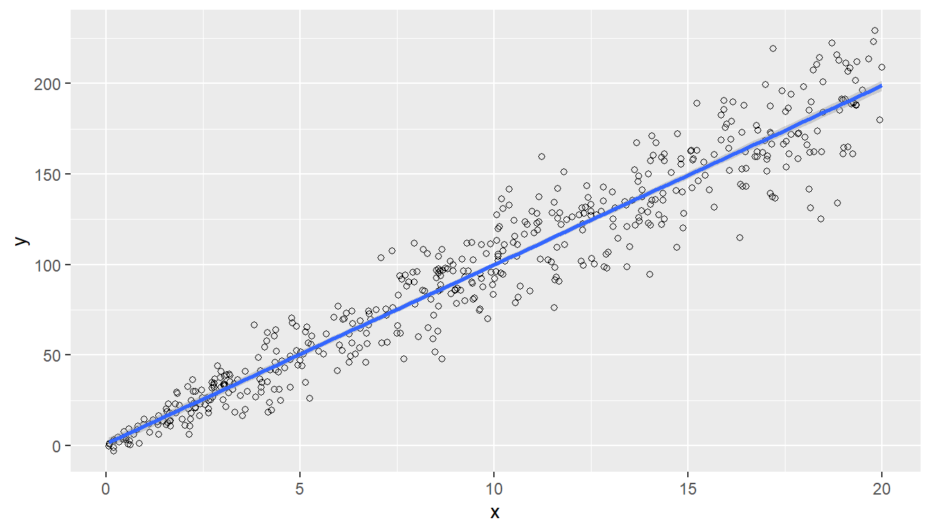

Figure 8.4: Scatterplot for a ratio model.

figure 8.4 shows the behavior of the relationship between the auxiliary information and the characteristic of interest. This model has the following properties: \[ \begin{aligned} E_{\xi}(Y_k)&=x_k'\beta \\ Var_{\xi}(Y_k)&=x_k\sigma^2. \end{aligned} \] The sample-based estimator of the regression coefficient is given by \[ \hat{B}=\left(\sum_S\frac{x_k}{\pi_k}\right)^{-1}\left(\sum_S\frac{y_k}{\pi_k}\right)=\frac{\hat{t}_{y,\pi}}{\hat{t}_{x,\pi}} \] Thus, under this model, the estimator of a ratio between two characteristics of interest is a special case of the regression coefficient.

Simple regression model without intercept: this model assumes the existence of a single continuous auxiliary information variable related to the characteristic of interest. It also assumes that the relationship must pass through the origin of the Cartesian plane and that the variance structure is constant. Thus \(p=1\), \(\mathbf{x}_k=x_k\), and \(c_k=1\) for all \(k\in U\). The model formulation is given by \[ Y_k=X_k'\beta+\varepsilon_k \] where each of the \(\varepsilon_k\), \(k\in U\), are independent and identically distributed random variables with mean zero and variance \(\sigma^2\).

N <- 1000
b <- 10
sigma <- 10

x <- runif(N, 0, 20)
e <- rnorm(N, 0, sigma)
y <- b * x + e

data <- data.frame(x, y)
ggplot(data, aes(x = x, y = y)) +
  geom_point(shape = 1) +
  geom_smooth(method = "lm")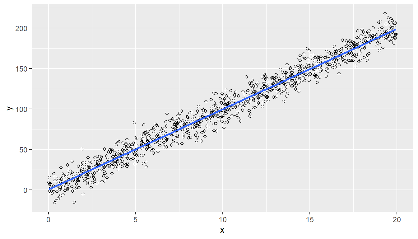

Figure 8.5: Scatterplot for a regression model without intercept.

figure 8.5 shows the behavior of the relationship between the auxiliary information and the characteristic of interest. This model has the following properties: \[ \begin{aligned} E_{\xi}(Y_k)&=x_k'\beta \\ Var_{\xi}(Y_k)&=\sigma^2. \end{aligned} \] The sample-based estimator of the regression coefficient is given by \[ \hat{B}=\left(\sum_S\frac{x_k^2}{\pi_k}\right)^{-1}\left(\sum_S\frac{x_ky_k}{\pi_k}\right)=\frac{\hat{t}_{xy,\pi}}{\hat{t}_{x^2,\pi}} \] It is important to emphasize that, like the ratio model, this model assumes that when the characteristic of interest takes the value zero, the continuous auxiliary information variable does so as well.

Simple regression model with intercept: this model assumes the existence of two continuous auxiliary information variables related to the characteristic of interest. One variable corresponds to the vector of ones, and the other corresponds to the continuous auxiliary information. With the inclusion of the vector of ones, the relationship is assumed not to pass through the origin. This model assumes that the variance structure is constant. Thus \(p=2\), \(\mathbf{x}_k=(1,x_k)'\), and \(c_k=1\) for all \(k\in U\). The model formulation is given by \[ \begin{aligned} Y_k&=\mathbf{X}_k'\boldsymbol{\beta}+\varepsilon_k \\ Y_k&=\beta_0+\beta_1X_k+\varepsilon_k \end{aligned} \] where each of the \(\varepsilon_k\), \(k\in U\), are independent and identically distributed random variables with mean zero and variance \(\sigma^2\). For this model, \(\boldsymbol{\beta}'=(\beta_0,\beta_1)\).

N <- 1000
a <- 200
b <- 10
sigma <- 10

x <- runif(N, 0, 20)
e <- rnorm(N, 0, sigma)
y <- a + b * x + e

data <- data.frame(x, y)
ggplot(data, aes(x = x, y = y)) +
  geom_point(shape = 1) +
  geom_smooth(method = "lm")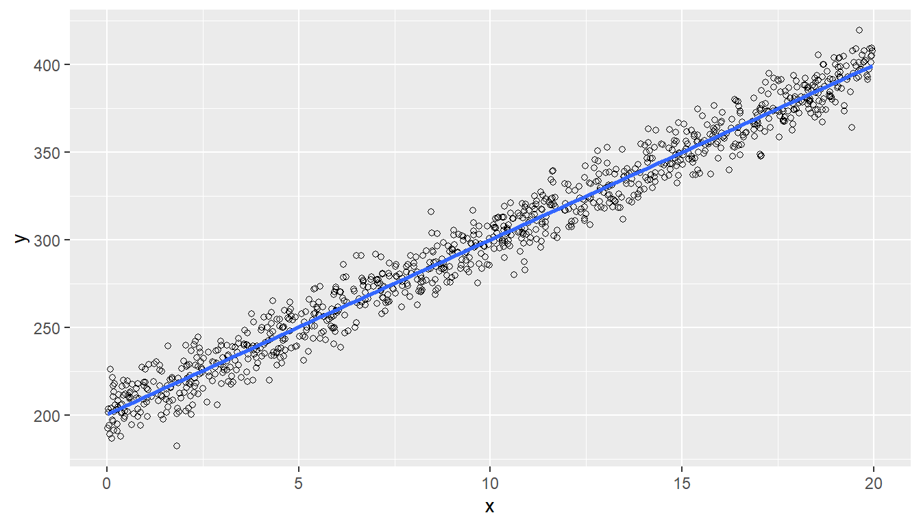

Figure 8.6: Scatterplot for a regression model with intercept.

figure 8.6 shows the behavior of the relationship between the auxiliary information and the characteristic of interest. This model has the following properties: \[ \begin{aligned} E_{\xi}(Y_k)&=\mathbf{x}_k'\boldsymbol{\beta}=\beta_0+\beta_1x_k \\ Var_{\xi}(Y_k)&=\sigma^2. \end{aligned} \] The sample-based estimator of the regression coefficient is given by \[ \hat{\mathbf{B}}=\begin{pmatrix} \hat{b}_0 \\ \hat{b}_1 \\ \end{pmatrix} \] where \[ \hat{b}_1=\dfrac{\sum_S\frac{(x_k-\widetilde{x}_S)(y_k-\widetilde{y}_S)}{\pi_k}}{\sum_S\frac{(x_k-\widetilde{x}_S)^2}{\pi_k}} \] and \[ \hat{b}_0=\widetilde{y}_S-\hat{b}_1\widetilde{x}_S \] Post-stratified mean model: this model assumes a partition of the finite population into \(G\) groups. Thus \(U=(U_1,U_2,\ldots,U_G)\). The characteristic of interest is assumed to be related to \(G\) vectors or dummy variables that take the value one if the element belongs to subgroup \(U_g\), \(g=1,\ldots,G\), and zero if the element does not belong to the group. Thus \(p=G\), \(\mathbf{x}_k=\mathbf{d}_k=(\underbrace{0,0,\ldots, 1, \ldots,0,0}_{G\text{ groups}})'\), and \(c_k=1\) for all \(k\in U\). The model formulation is given by \[ Y_k=\mathbf{d}_k'\boldsymbol{\beta}+\varepsilon_k=\beta_g+\varepsilon_k \ \ \ \ \quad g=1,\ldots,G. \] where \(\boldsymbol{\beta}=(\beta_1,\ldots,\beta_g,\ldots,\beta_G)'\) and each of the \(\varepsilon_k\), \(k\in U\), are independent and identically distributed random variables with mean zero and variance \(\sigma^2_g\). Note that \(\mathbf{d}_k=(d_{1k},\ldots,d_{gk},\ldots,d_{Gk})'\) with \[ d_{gk}= \begin{cases} 1, & \text{if } k\in U_g\\ 0, & \text{otherwise.} \end{cases} \]

N <- 1000
b1 <- 10
b2 <- 20
b3 <- 5

x <- runif(N, 0, 20)
e <- rnorm(N, 0, 1)
y1 <- b1 + e
y2 <- b2 + e
y3 <- b3 + e

data <- data.frame(x, y1, y2, y3)
p1 <- ggplot(data, aes(x = x, y = y1)) +
  geom_point(shape = 1) +
  geom_smooth(method = "lm") +
  ylim(0, 25) +
  ggtitle("Group 1")
p2 <- ggplot(data, aes(x = x, y = y2)) +
  geom_point(shape = 1) +
  geom_smooth(method = "lm") +
  ylim(0, 25) +
  ggtitle("Group 2")
p3 <- ggplot(data, aes(x = x, y = y3)) +
  geom_point(shape = 1) +
  geom_smooth(method = "lm") +
  ylim(0, 25) +
  ggtitle("Group 3")
grid.arrange(p1, p2, p3, ncol = 3)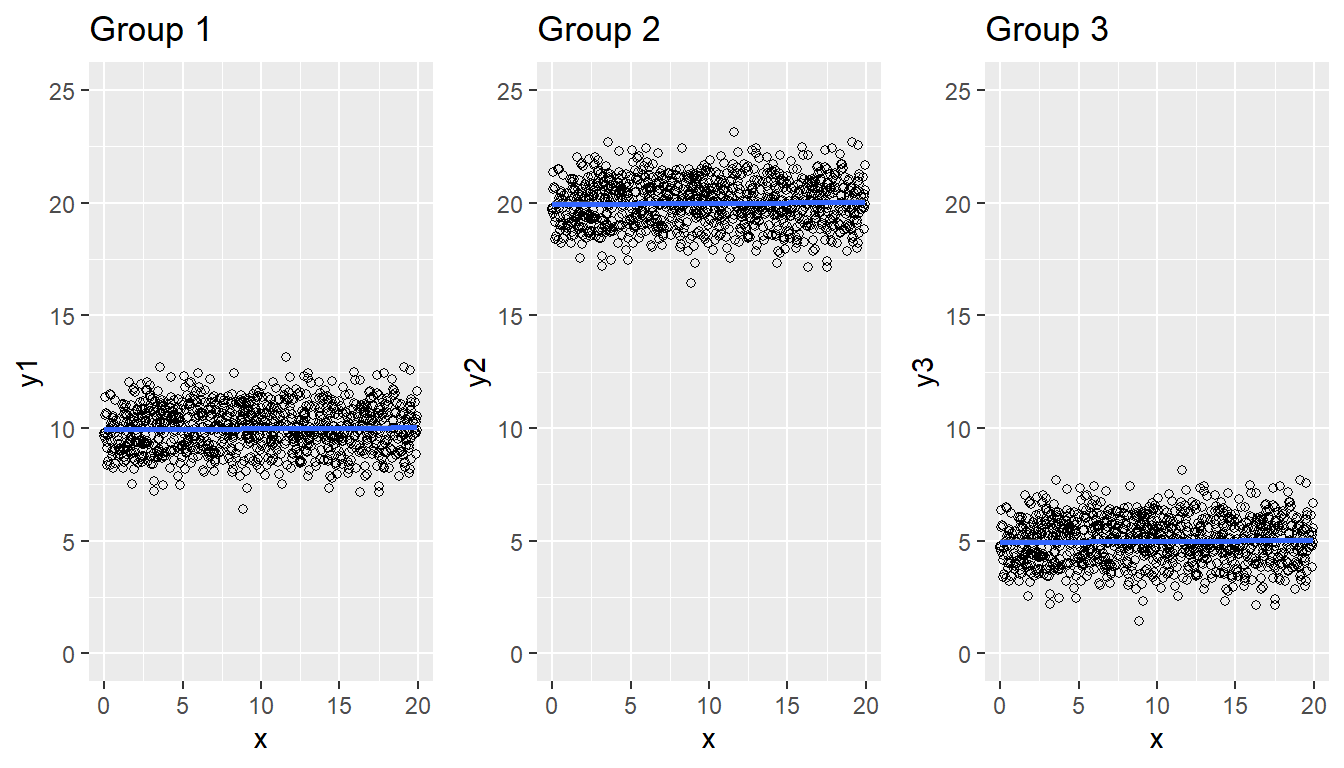

Figure 8.7: Scatterplot for a post-stratified mean model.

figure 8.7 shows the behavior of the relationship between the auxiliary information and the characteristic of interest. This model has the following properties: \[ \begin{aligned} E_{\xi}(Y_k)&=\mathbf{d}_k'\boldsymbol{\beta}=\beta_g+\varepsilon_k \\ Var_{\xi}(Y_k)&=\sigma^2_g. \end{aligned} \tag{8.4}\] The sample-based estimator of the regression coefficient is given by \[ \hat{\mathbf{B}}=(\hat{B}_1,\hat{B}_2,\ldots,\hat{B}_G)' \] where \[ \hat{{B}}_g=\left(\sum_{S_g}\frac{1}{\pi_k}\right)^{-1}\left(\sum_{S_g}\frac{y_k}{\pi_k}\right)= \frac{\hat{t}_{yU_g,\pi}}{\hat{N}_{U_g,\pi}}=\widetilde{y}_{S_g} \] Post-stratified ratio model: this model assumes a partition of the finite population into \(G\) groups, so that \(U=(U_1,U_2,\ldots,U_G)\). It is assumed that a ratio model can be defined in each of the subgroups \(U_g\), \(g=1,\ldots,G\). Thus, the ratio between the characteristic of interest and the auxiliary information is considered constant within each subgroup but different across subgroups. Then \(p=G\), \(\mathbf{x}_k=\mathbf{d}_kx_k=(\underbrace{0,0,\ldots, x_k, \ldots,0,0}_{G\text{ groups}})'\), and \(c_k=x_k\) for all \(k\in U_g\). The model formulation is given by \[ Y_k=\beta_gX_k+\varepsilon_k \ \ \ \ \quad g=1,\ldots,G. \] where each of the \(\varepsilon_k\), \(k\in U_g\), are independent and identically distributed random variables with mean zero and variance \(\sigma^2_g\) for \(g=1,\ldots,G\).

N <- 500
b1 <- 2
b2 <- 1
b3 <- 0.5

x <- runif(N, 0, 20)
e <- rnorm(N, 0, 1)
y1 <- b1 * x + e
y2 <- b2 * x + e
y3 <- b3 * x + e

data <- data.frame(x, y1, y2, y3)
p1 <- ggplot(data, aes(x = x, y = y1)) +
  geom_point(shape = 1) +
  geom_smooth(method = "lm") +
  ylim(0, 25) +
  ggtitle("Group 1")
p2 <- ggplot(data, aes(x = x, y = y2)) +
  geom_point(shape = 1) +
  geom_smooth(method = "lm") +
  ylim(0, 25) +
  ggtitle("Group 2")
p3 <- ggplot(data, aes(x = x, y = y3)) +
  geom_point(shape = 1) +
  geom_smooth(method = "lm") +
  ylim(0, 25) +
  ggtitle("Group 3")
grid.arrange(p1, p2, p3, ncol = 3)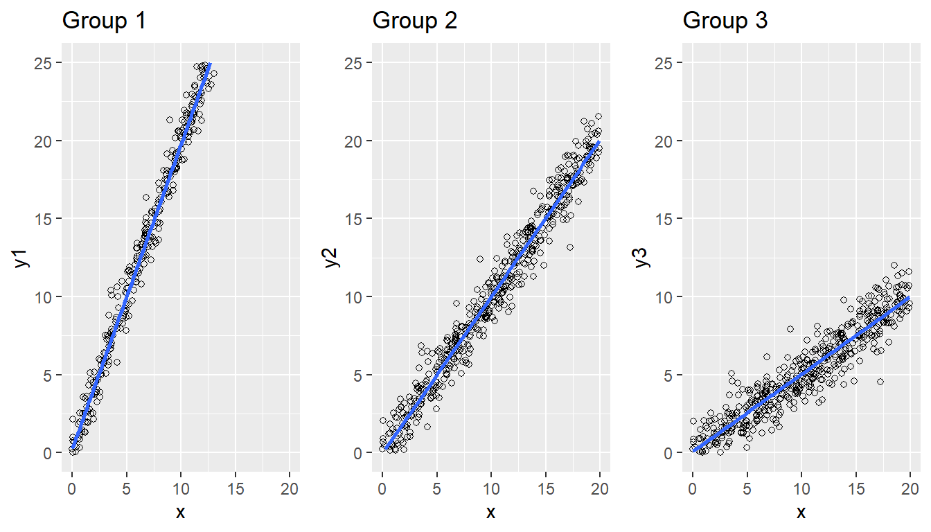

Figure 8.8: Scatterplot for a post-stratified ratio model.

figure 8.8 shows the behavior of the relationship between the auxiliary information and the characteristic of interest. This model has the following properties: \[ \begin{aligned} E_{\xi}(Y_k)&=\beta_gx_k \\ Var_{\xi}(Y_k)&=x_k\sigma^2_g. \end{aligned} \tag{8.5}\] The sample-based estimator of the regression coefficient is given by \[ \hat{\mathbf{B}}=(\hat{B}_1,\hat{B}_2,\ldots,\hat{B}_G)' \] where \[ \hat{\mathbf{B}}_g=\left(\sum_{S_g}\frac{x_k}{\pi_k}\right)^{-1}\left(\sum_{S_g}\frac{y_k}{\pi_k}\right)= \frac{\hat{t}_{yU_g,\pi}}{\hat{t}_{xU_g,\pi}} \] There are more models, but the preceding ones are the most commonly used in practice. The proof of the preceding expressions is left as an exercise for the reader.

Example

Returning to our example population \(U\), suppose that we have access to the values of the characteristic of interest \(y\) and the continuous auxiliary information \(x\). In addition, suppose that the model governing the relationship between the two is given by \[ Y_k=\beta_0+\beta_1X_k+\varepsilon_k \] where each of the \(\varepsilon_k\), \(k\in U\), are independent and identically distributed random variables with mean zero and constant variance. By estimating \(\beta_0\) and \(\beta_1\) using the least squares method, we obtain the model formulation in the finite population. For this, we use the lm function from the R computing environment.

N <- 5
x <- c(32, 34, 46, 89, 35)
y <- c(52, 60, 75, 100, 50)
lm(y ~ x)


Call:
lm(formula = y ~ x)

Coefficients:
(Intercept)            x  
     28.505        0.824

This leads us to conclude that, in the hypothetical case of having access to all data from the finite population, the estimated model would be \[ y_k=28.505+0.824x_k+E_k \] Of course, in practice we do not have access to the finite population; therefore, through a sampling design we select a sample of size \(n=4\). The sampling design induces inclusion probabilities pik for each of the elements. Suppose that the selected sample consists of the first four elements of the population; that is, Yves, Ken, Erik, and finally Sharon. Therefore, the information collected after the measurement process is stored in the vectors x.s and y.s; likewise, the inclusion probabilities of the elements included in the sample are stored in pik.s.

pik <- c(1, 0.5, 1, 1, 0.5)
sam <- c(1, 2, 3, 4)
n <- length(sam)
x.s <- x[sam]
y.s <- y[sam]
pik.s <- pik[sam]

To carry out the estimation taking into account the sampling weights, defined as \(1 / \pi_k\), it is enough to use the lm function and ensure that the weights option is properly defined.

lm(y.s ~ x.s, weights = 1 / pik.s)


Call:
lm(formula = y.s ~ x.s, weights = 1/pik.s)

Coefficients:
(Intercept)          x.s  
     33.363        0.767

Assuming that the sampling had been simple random sampling without replacement, it is possible to use the E.Beta function from the TeachingSampling package, which estimates regression coefficients under any proposed model using the information collected in the sample. The E.Beta function has four parameters: y, the data set containing the values of the characteristic(s) of interest in the sample; x, the design matrix or matrix containing the continuous or discrete auxiliary information. This argument may be a vector, in the case of a single auxiliary information variable, or a matrix, in the case of multiple auxiliary information. pik is the vector of inclusion probabilities for the elements included in the sample. b0, which by default takes the value FALSE, indicates that the model was proposed without an intercept. Otherwise, if the proposed model contains an intercept, b0 must take the value TRUE. The last function argument is ck, which refers to the model variance structure; ck takes the value 1 by default. If the variance structure is like that of the ratio model, then ck should be the same vector introduced in the x argument.

E.Beta(N, n, as.data.frame(y.s), x.s, b0 = TRUE, ck = 1)

, , y.s

                  V1     x
Beta estimation 33.0 0.771
Standard Error   2.4 0.031
CVE              7.3 3.959

In this case, the estimation based on the information collected in the sample gives an intercept of \(\hat{B}_0=33.36\) and a regression-line slope of \(\hat{B}_1=0.77\). The model formulation at the sample level would be: \[ y_k=33.36+0.77x_k+e_k \] Since ratio estimation and the weighted mean are special cases of regression coefficient estimation, the E.Beta function easily allows these estimates to be computed by setting its parameters appropriately.

8.4.5 Marco y Lucy

It is of vital interest for government collaborators to know the relationship between the characteristics of interest, because these relationships allow them to formulate econometric models that provide deeper insight into the sector’s behavior in the last fiscal year. If population information were available and the researchers were interested in formulating a different model for each characteristic of interest: number of Employees and Taxes declared in the last fiscal year with respect to Income obtained in the same period.

Below we present the reasoning that leads us to choose the appropriate regression model for each variable. The continuous auxiliary information is the Income characteristic, while the characteristics of interest related to it are Employees and Taxes. Does it make sense to fit both models with an intercept? Consider the following extreme scenario that may occur: a firm has zero income during the year but continues operating with help from the government, a capital injection from another firm, or simply its own capital reserves. Therefore, zero income does not mean that the firm has zero employees, so the model to be fitted may need an intercept. On the other hand, if income is zero, the firm’s tax declaration will also be zero. That is, the model fitted for this characteristic of interest should not contain an intercept parameter.

Thus, using the least squares method, we would be able to formulate the two models needed to answer the researchers’ objectives. We fit the regression using the lm function. The variance structure for each model is assumed to be constant.

data(BigLucy)
y1 <- as.matrix(BigLucy$Employees)
y2 <- as.matrix(BigLucy$Taxes)
x <- as.matrix(BigLucy$Income)

m1 <- lm(y1 ~ x)
m1


Call:
lm(formula = y1 ~ x)

Coefficients:
(Intercept)            x  
    29.1244       0.0794

m2 <- lm(y2 ~ x - 1)
m2


Call:
lm(formula = y2 ~ x - 1)

Coefficients:
     x  
0.0363

Thus, the models fitted in the finite population for the two characteristics of interest would be \[ \begin{aligned} Employees_k &= 29.12 + 0.08 \times Income_k +E_k\\ \\ Taxes_k &= 0.04 \times Income_k + E_k \end{aligned} \] Of course, the preceding models would be fitted to the population. In practice, we do not have access to all values taken by the characteristics of interest, which is why we must estimate the regression coefficients. Suppose that the sampling was simple random sampling without replacement, with a sample size of \(n=2000\) firms.

N <- dim(BigLucy)[1]
n <- 2000
sam <- S.SI(N, n)
sample_data <- BigLucy[sam, ]

To estimate the regression coefficients, the E.Beta function from the sampling package must be used. For the model with intercept for the Employees characteristic, the function parameters are set so that they align with the model assumptions: note that b0 takes the value TRUE and, because of the variance structure, ck takes the value 1. On the other hand, for the model without intercept for the Taxes characteristic, b0 must be FALSE; as in the previous model, ck still takes the value 1.

E.Beta(N, n, as.matrix(sample_data$Employees), sample_data$Income, b0 = TRUE, ck = 1)

, , 1

                  V1      x
Beta estimation 29.0 0.0803
Standard Error   1.1 0.0024
CVE              3.9 2.9360

E.Beta(N, n, as.matrix(sample_data$Taxes), sample_data$Income, b0 = FALSE, ck = 1)

, , 1

                  [,1]
Beta estimation 0.0385
Standard Error  0.0019
CVE             5.0476

Thus, the models estimated in the finite population are \[ \begin{aligned} Employees_k &= 25.43+0.087\times Income_k+e_k\\ \\ Taxes_k &= 0.037\times Income_k+e_k \end{aligned} \] Broadly speaking, this estimate indicates that, with zero income, firms have on average 25 employees; that for every 11.7 increase in income one employee is hired; and that, on average, firms pay a tax rate of 3.7% to the government. Note that if the model had been a ratio model, then the function required to estimate the regression coefficient, which coincides with the estimation of a ratio, would be:

E.Beta(N, n, as.matrix(sample_data$Taxes), sample_data$Income, b0 = FALSE, ck = sample_data$Income)

, , 1

                    [,1]
Beta estimation    0.028
Standard Error     1.349
CVE             4821.555

8.5 Exercises

Carry out the lexicographic exercise from Example 8.3.1. Use this exercise to illustrate whether the estimator \(\hat{M}\) is unbiased or not.
With the data from the previous exercise, select a sample of size \(n=4\). Use Result 8.3.1 to obtain an estimate of the distribution function and plot your findings.
To estimate the total of the characteristic of interest for a population of N = 284 elements, a Poisson sampling design with expected sample size \(n(S) = 10\) was used. The inclusion probabilities were proportional to an auxiliary information characteristic \(x\) whose population total is \(t_x = 8182\). The selection algorithm yielded an effective sample size of 12 elements, for which the information from Exercise 4.5 was obtained. Estimate the median and the distribution function for the characteristic of interest.
Suppose that the data from the previous exercise were obtained using a simple random sampling design. Estimate the difference of totals \(t_y-t_x\) using \(\hat{t}_{y-x}=\hat{t}_{y,\pi}-\hat{t}_{x,\pi}\). Estimate the variance and calculate the estimated coefficient of variation.
Suppose that the data from the previous exercise were obtained using a Bernoulli sampling design with \(\pi=0.04\).
Estimate the ratio of totals \(t_y/t_x\) using \(\hat{B}=\hat{t}_{y,\pi}/\hat{t}_{x,\pi}\). Estimate the variance and calculate the estimated coefficient of variation.
Estimate the mean of the characteristic of interest using the Hájek estimator. Estimate the variance and calculate the estimated coefficient of variation.
Estimate the mean of the auxiliary information characteristic using the Hájek estimator. Estimate the variance and calculate the estimated coefficient of variation.
Verify the expression for the variance matrix \(AV(\hat{\mathbf{B}})\).
In a sample of municipalities, based on a simple random sampling design, \(n=10\) municipalities were selected from \(N=49\). In each municipality, the following characteristics were measured: the number of inhabitants in the municipality (HAB), the number of automobiles in the municipality (VEH), and the number of military personnel in the municipality (MIL). In addition, each municipality is known to be categorized (CAT) as urban (CAT=1) or rural (CAT=0). The information collected from the municipalities in the sample is shown below:

HAB	VEH	MIL	CAT
2571	50	415	1
2813	55	462	1
3002	61	513	1
3564	70	577	1
3051	64	532	0
2835	56	463	0
3319	67	551	0
2986	61	512	0
2998	55	471	0
2717	56	462	0

Estimate the regression coefficient of HAB against VEH for a common mean model. Estimate the variance and calculate the coefficient of variation. Interpret the estimated coefficient.
Estimate the regression coefficient of HAB against VEH for a ratio model. Estimate the variance and calculate the coefficient of variation. Interpret the estimated coefficient.
Estimate the regression coefficients of HAB against MIL for a simple regression model with intercept. Estimate the variance matrix and calculate the coefficients of variation. Interpret the estimated coefficients.
Estimate the regression coefficients of HAB against CAT for a post-stratified mean model. Estimate the variance matrix and calculate the coefficients of variation. Interpret the estimated coefficients.
Estimate the regression coefficients of HAB against MIL for a post-stratified ratio model using CAT. Estimate the variance matrix and calculate the coefficients of variation. Interpret the estimated coefficients.
Support or refute the following statements.
A linear function of unbiased estimators is always unbiased for its population counterpart.
An estimator is said to be approximately unbiased when it is biased only for the linear part of the Taylor expansion.
In estimating a population ratio \(B\), the linearized variable \(E_k=\frac{1}{t_z}(y_k-Bz_k)\) satisfies \(\sum_S E_k =0\) regardless of the sampling design used in planning the study.
The estimator \(\hat{B}=\frac{\hat{t}_{y,\pi}}{\hat{t}_{z,\pi}}\) is biased for \(B=\frac{t_y}{t_z}\) only if \(z_k\) is continuous.
In sampling designs with random sample size, the estimator of the population mean \(\tilde{y}_S\) is unbiased and has smaller variance than the estimator \(\bar{y}_S\).
The Taylor linearization method for approximating the variance of complex parameters in small samples generally leads to overestimation of the true variance.
The estimator \(\hat{\mathbf{B}}=\hat{\mathbf{T}}^{-1}\hat{\mathbf{t}}\) is always biased for \(\mathbf{B}=\mathbf{T}^{-1}\mathbf{t}\) regardless of the quality of the fit.
For the Hajek estimator, defined as \(\tilde{y}_S=\hat{t}_{y,\pi}/\hat{N}_{\pi}\), and using the Taylor linearization technique, show that this estimator is approximately unbiased for \(\bar{y}_U=t_y/N\) and propose an expression for the approximate variance estimator.
For the alternative total estimator, defined as \(\hat{t}_{y,alt}=N\tilde{y}_S\), and using the Taylor linearization technique, show that this estimator is approximately unbiased for \(t_y=\sum_Uy_k\) and propose an expression for the approximate variance estimator.
For a two-stage sampling design in which the first stage uses a with-replacement PPS design and the second stage uses an SRS design within each selected PSU, propose an approximately unbiased estimator for the population ratio and define the variance for this estimator.
State whether the following statements are false or true. Justify your answer in detail.
A linear function of unbiased estimators is always unbiased for its population counterpart.
An estimator is said to be approximately unbiased when it is biased only for the linear part of the Taylor expansion.
The estimator \(\hat{B}=\frac{\hat{t}_{y,\pi}}{\hat{t}_{z,\pi}}\) is biased for \(B=\frac{t_y}{t_z}\) only if \(z_k\) is continuous.
In sampling designs with random sample size, the estimator of the population mean \(\tilde{y}_S\) is unbiased and has smaller variance than the estimator \(\bar{y}_S\).
In estimating a population ratio \(B\), the linearized variable \(E_k=\frac{1}{t_z}(y_k-Bz_k)\) satisfies \(\sum_S E_k =0\) regardless of the sampling design used in planning the study.
The estimator \(\hat{B}=\frac{\hat{t}_{y,\pi}}{\hat{t}_{z,\pi}}\) is biased for \(B=\frac{t_y}{t_z}\) only if \(z_k\) is continuous.
In sampling designs with random sample size, the estimator of the population mean \(\tilde{y}_S\) is unbiased and has smaller variance than the estimator \(\bar{y}_S\).
The Taylor linearization method for approximating the variance of complex parameters in small samples generally leads to overestimation of the true variance.
Consider Exercise 7.4.
Estimate the number of people in the country, \(\hat{N}\). Report the estimated coefficient of variation.
Estimate mean income in the country using the Hajek ratio \(\tilde{y}_S=t_{y,\pi}/\hat{N}\). Report the estimated coefficient of variation.
Consider Exercise 7.5.
If the northern zone was selected, report the estimate of the average number of legs in the city using the Hájek ratio \(\tilde{y}_S=t_{y,\pi}/\hat{N}\).
If the northern zone was selected, report the estimate of the average number of legs in the city using the Hájek ratio \(\tilde{y}_S=t_{y,\pi}/\hat{N}\).
For this sampling design, report the variance approximation of the estimator \(\bar{y}_S\).
Which estimator would you choose to infer about the average number of dogs’ legs in the city? \(\bar{y}_S\) or \(\tilde{y}_S\)?
Is it better to account for N, or is it better to estimate it using \(\hat{N}\)?

Apostol, T. M. 1963. Mathematical Analysis. Adison Wesley.

Bautista, J. L. 1998. Diseños de Muestreo Estad’istico. Universidad Nacional de Colombia.

Binder, D. 1983. “On the Variances of Asymptotically Normal Estimators from Complex Surveys.” International Statistical Review 51: 279–92.

Breidt, F. J., and J. D. Opsomer. 2000. “Local Polynomial Regression Estimators in Survey Sampling.” The Annals of Statistics 28: 1026–53.

Cassel, C. M., C. E. Särndal, and J. Wretman. 1976. Foundations of Inference in Survey Sampling. Wiley.

Deville, J-C. 1999. “Variance Estimation for Complex Statistics and Estimators: Linearizaion and Residual Techniques.” Survey Methodology 25: 193–204.

Draper, D. 1998. “Rank-Based Robust Analysis of Linear Models i. Exposition and Review.” Statistical Science 3: 239–57.

Gutiérrez, H. A. 2009. “Model Assisted Survey Regression Estimators: A Rank-Based Approach.” Proceedings of the 57th Session of the International Statistical Institute, 18–31.

Gutiérrez, H. A., and F. J. Breidt. 2009. “Estimation of the Population Total Using the Generalized Difference Estimator and Wilcoxon Ranks.” Revista Colombiana de Estadística 32: 123–43.

Lohr, S. 2000. Sampling: Design and Analysis. Thompson.

Madow, W. 1948. “On the Limiting Distributions Based on Samples from Finite Universes.” Annals of Mathematical Statistics 19: 535–45.

Ravishanker, N., and D. Dey. 2002. A First Course in Linear Model Theory. Chapman; Hall.

Rosén, B. 1972. “Asymptotic Theory for Succesive Sampling with Varying Probabilities Without Replacement, i and II.” Annals of Mathematical Statistics 43: 373–97, 748–76.

Särndal, C. E., B. Swensson, and J. Wretman. 1992. Model Assisted Survey Sampling. Springer, New York.

Woodruff, R. 1971. “A Simple Method for Approximating the Variance of a Complicated Estimate.” Journal of the American Statistical Association 66: 411–14.

Under the assumption that the election would take place on the same day as the interview.↩︎
Of course, the sampling design may vary. If a two-stage random design had been used, the functions to use would be S.SI to select the sample and E.2SI to carry out the estimation.↩︎
A population value for which \(q\%\) of the values of the characteristic of interest in the population satisfy \(y_k\leq y\).↩︎
Draper (1998) states that to calculate a weighted median, the observations must be ordered from smallest to largest, carrying their weights along that ordering. Then the total sum \(\Sigma\) of the weights must be found, and the weights must be added from top to bottom until \(\Sigma/2\) is reached.↩︎
This alternative procedure is computationally much simpler.↩︎
In this PPS sampling case, we use expression (2.2.19) to compute the \(\pi_k\) from the \(p_k\).↩︎
This model is known as the superpopulation model between \(Y\) and \(\mathbf{X}\).↩︎
The statistical properties of these random variables must be considered under the model \(\xi\).↩︎