Chapter 3 Analysis of continuous variables
The statistical analysis of surveys has constantly evolved, driven by the development of new methodologies and approaches that seek to improve the precision and representativeness of the results. In general, these advances emerge in the academic field and, over time, are adopted by public institutions, private companies and statistical organizations, which demand their incorporation into the main data analysis programs.
This chapter presents the main procedures for the statistical analysis of continuous variables using R, appropriately incorporating the characteristics of the sampling design, such as expansion weights, stratification and conglomeration. Throughout the chapter, methods are illustrated to estimate population parameters, measure their precision, and make valid inferences from data from complex surveys. Likewise, functions and tools of the survey (Lumley, 2024) package are introduced, one of the most used resources in R for survey analysis.
Databases used in survey analysis can be found in a wide variety of formats (.xlsx, .dat, .csv, .parquet, .sas7bdat, .sav, .txt, among others). However, a good practice is to import the information from any of these formats and immediately save it in a file with the extension .rds, which is the native format of R.
.rds files allow you to store any object or information in R, such as data frames, vectors, matrices or lists, and are characterized by their complete compatibility with the R work environment. In addition, they facilitate efficient reading and writing of data, reducing loading times and avoiding compatibility problems between sessions. Another R format is .Rdata, which allows multiple objects to be saved in a single file. In contrast, .rds files store only one object, making their use more controlled and reproducible. For this reason, it is recommended to preferably work with the .rds format when documenting projects or reproducing analyses.
To illustrate the computational syntax that will be used throughout the chapter, we use the same database as in the previous chapter, which contains a sample of 2,605 records from a complex sample design. The following shows how to load a file with the .rds extension:
According to Naciones Unidas (2009, Section 7.8), it is essential that the structure of the sampling design be taken into account in the inference process when estimating official statistics based on household surveys. As emphasized in this document, ignoring this aspect can generate biased estimates and underestimated sampling errors. In this sense, statistical programs incorporate specific functionalities to handle data from surveys with complex designs (Heeringa et al., 2017, appendix A).
Once the sample of households has been loaded into R, the next step is to define the sample design from which said sample comes. For this, the srvyr (Freedman Ellis & Schneider, 2024) package will be used, which appears as a complement to the survey (Lumley, 2024) package. These libraries allow defining survey.design type objects, to which the estimation and survey analysis functions are applied, and which can be combined with the programming of the tidyverse (Wickham, Averick, et al., 2026) package. Here is an example of defining an object of type survey_design for the survey:
options(survey.lonely.UPM = "adjust")

library(survey)
library(srvyr)

survey_design <- survey_data %>%
  as_survey_design(
    strata = Stratum,
    ids = PSU,
    weights = wk,
    nest = TRUE
  )
In this code, survey_data corresponds to the database that contains the selected sample. From this data, the function as_survey_design() converts the information into an object of class survey_design, which stores all the elements necessary to describe the sample design of the survey. These include the stratification variable (strata), which identifies the strata defined in the design, and the variable specified in ids, which represents the primary sampling units (PSUs) or clusters selected in the first stage of sampling. Likewise, the weights argument defines the variable that contains the expansion factors associated with each observation. Finally, the nest = TRUE option indicates that PSUs are nested within strata, a necessary characteristic to correctly represent the hierarchical structure of the sampling design.
## Estimation of descriptive parameters {#estimacion-de-parametros-descriptivos}
In household surveys it is common to estimate descriptive parameters associated with numerical variables, such as totals, means, ratios and standard deviations. These measures allow us to characterize different social and economic phenomena of the population, for example income, expenditure, hours worked or household size. This section presents the logic behind the syntax used for this type of estimation, along with its corresponding precision measures. ### Total estimate {#estimacion-del-total}
In R, the survey_total() function is used to estimate totals from the design object. This feature automatically incorporates expansion factors and design structure, ensuring that estimates correctly reflect the inference model.
The main arguments of the survey_total() function are x, na.rm, vartype, level, and deff. The x argument corresponds to the variable on which you want to calculate the total; It can also be left empty when seeking to obtain only the weighted total of cases in the sample. Meanwhile, na.rm indicates whether missing values (NA) should be removed before performing the calculation, with FALSE being the default value.
The vartype argument allows you to specify the type of uncertainty measure that you want to estimate, and one or more results can be requested simultaneously, such as the standard error ("se"), the confidence interval ("ci"), the variance ("var") or the coefficient of variation ("cv"). Likewise, level defines the confidence level used to calculate the confidence intervals, whose default value is 0.95. On the other hand, the confidence interval can be obtained directly by including the argument vartype = "ci" within survey_total(), or by using the function confint() on the resulting object, specifying the required confidence level. Finally, deff is a logical value that indicates whether to return the design effect (DEFF).
The following example presents how to estimate totals and their confidence intervals for different variables of interest in R, using the function survey_total(), and presented in Table 3.1:
| total | total_se | total_low | total_upp | total_deff |
|---|---|---|---|---|
| 85793667 | 4778674 | 76331414 | 95255920 | 11 |
From the table, it is obtained that the estimate of the total population for the total income is 85,793,667. This value corresponds to the point estimator obtained from the survey, incorporating the expansion factors and the characteristics of the sample design. The standard error associated with this estimate is 4,778,674, which reflects the sample variability of the estimator. From this value, a 95% confidence interval is constructed, whose lower and upper limits are 76,331,414 and 95,255,920, respectively. The design effect (deff) is equal to 11, suggesting a significant loss of accuracy mainly associated with complex design characteristics. Consequently, although the nominal sample size may be large, the effective sample size would be considerably smaller due to the correlation between observations within the clusters.
To continue illustrating the use of the survey_total() function within the srvyr approach, let us estimate total household expenditures, but now calculating the 90% confidence interval. The following code performs this estimation, presented in Table 3.2:
survey_design %>%
  summarise(total = survey_total(Expenditure,
                              vartype = "ci", level = 0.9,
deff = TRUE))| total | total_low | total_upp | total_deff |
|---|---|---|---|
| 55677504 | 51360469 | 59994539 | 10.2 |
If the objective is to estimate total household income, but disaggregated by sex, the function group_by() can be used to group by the variable of interest, together with cascade() from the srvyr library, which allows adding a row with the general total at the end of the table. In this way, category totals and the overall total can be easily obtained within the same summary framework, as shown in Table 3.3.
survey_design %>%
  group_by(Sex) %>%
  cascade(total = survey_total(Income,
                               vartype = c("se", "ci"),
                               level = 0.95),
.fill = "Total income")| Sex | total | total_se | total_low | total_upp |
|---|---|---|---|---|
| Female | 44153820 | 2324452 | 39551172 | 48756467 |
| Male | 41639847 | 2870194 | 35956576 | 47323118 |
| Total income | 85793667 | 4778674 | 76331414 | 95255920 |
As seen in the previous codes, a practical way to obtain the estimates of the total, its standard error and its confidence interval is through the argument vartype, specifying the options "se" and "ci" respectively.
### Estimation of the mean {#estimacion-de-la-media}
The estimation of the population average occupies a central place in household surveys, since many of the indicators used for socioeconomic analysis correspond to average values, such as average household income, per capita spending or average hours worked. This type of parameters allows us to summarize the general behavior of the variables of interest and describe the central tendencies of the target population. According to Gutiérrez (2016), the population mean estimator can be expressed as a non-linear ratio between two population totals, which are estimated as follows: \[ \hat{\bar{y}}= \frac{\hat{t}_y}{\hat{N}} = \frac{\sum_{h}\sum_{i}\sum_{k} w_{h i k} \ y_{hik}}{\sum_{h}\sum_{i}\sum_{k} w_{h i k}} \]
Since \(\hat{\bar{y}}\) is not a linear statistic, there is no closed formula for the variance of this estimator. For this reason, it is necessary to resort to resampling methods or Taylor linearization to approximate its variance. In this particular case, using Taylor series, the variance is defined as: \[ \widehat{Var}\left(\hat{\bar{y}}\right) \approx \frac{\widehat{Var}\left(\hat{t}_y\right)+\hat{\bar{y}}^{2}\ \widehat{Var}\left(\hat{N}\right)-2\ \hat{\bar{y}} \ \widehat{Cov}\left(\hat{t}_y,\hat{N}\right)}{\hat{N}^{2}} \]
As can be seen, the calculation of the variance of the population mean involves complex analytical components, such as the covariance between the estimated total and the estimated population size. However, the srvyr package in R facilitates these calculations by incorporating functions that directly estimate the mean, its standard error, the confidence interval, and the design effect. Below is the syntax to estimate the average household income, along with its 95% confidence interval, presented in Table 3.4:
survey_design %>%
  summarise(mean = survey_mean(Income,
                                vartype = c("se", "ci"),
                                level = 0.95,
deff = TRUE))| mean | mean_se | mean_low | mean_upp | mean_deff |
|---|---|---|---|---|
| 571 | 28.5 | 515 | 627 | 8.82 |
As can be seen, the arguments used in the survey_mean() function are similar to those of survey_total(). In this case, vartype allows you to obtain the standard error ("se") and the confidence interval ("ci"), while the argument deff = TRUE requests the calculation of the design effect. Similarly, it is possible to estimate the average household expenses, using the same code structure, presented in Table 3.5:
survey_design %>%
  summarise(mean = survey_mean(Expenditure,
                                    vartype = c("se", "ci"),
                                    level = 0.95,
deff = TRUE))| mean | mean_se | mean_low | mean_upp | mean_deff |
|---|---|---|---|---|
| 371 | 13.3 | 344 | 397 | 6.02 |
Estimates of the mean by subgroups can also be made following the same scheme shown previously. Particularly, household expenses discriminated by sex are presented in Table 3.6:
survey_design %>%
  group_by(Sex) %>%
  cascade(mean = survey_mean(Expenditure,
                              level = 0.95,
                              vartype = c("se", "ci")),
        .fill = "Mean expenditure") %>%
arrange(desc(Sex))| Sex | mean | mean_se | mean_low | mean_upp |
|---|---|---|---|---|
| Mean expenditure | 371 | 13.3 | 344 | 397 |
| Male | 374 | 16.1 | 343 | 406 |
| Female | 367 | 12.3 | 343 | 391 |
In an analogous manner, the average expenditure by area can be calculated, which is presented in Table 3.7:
survey_design %>%
  group_by(Zone) %>%
  cascade(mean = survey_mean(Expenditure,
                              level = 0.95,
                              vartype = c("se", "ci")),
        .fill = "Mean expenditure") %>%
arrange(desc(Zone))| Zone | mean | mean_se | mean_low | mean_upp |
|---|---|---|---|---|
| Urban | 460 | 22.2 | 416 | 504 |
| Rural | 274 | 10.3 | 254 | 294 |
| Mean expenditure | 371 | 13.3 | 344 | 397 |
Likewise, it is possible to make a combined estimate by sex and area, presented in Table 3.8:
survey_design %>%
  group_by(Zone, Sex) %>%
  cascade(mean = survey_mean(Expenditure,
                              level = 0.95,
                              vartype = c("se", "ci")),
        .fill = "Mean expenditure") %>%
arrange(desc(Zone), desc(Sex))| Zone | Sex | mean | mean_se | mean_low | mean_upp |
|---|---|---|---|---|---|
| Urban | Mean expenditure | 460 | 22.2 | 416 | 504 |
| Urban | Male | 470 | 27.0 | 416 | 523 |
| Urban | Female | 451 | 20.1 | 411 | 491 |
| Rural | Mean expenditure | 274 | 10.3 | 254 | 294 |
| Rural | Male | 275 | 10.2 | 255 | 296 |
| Rural | Female | 273 | 11.6 | 250 | 296 |
| Mean expenditure | Mean expenditure | 371 | 13.3 | 344 | 397 |
3.0.1 Ratio estimation
A particular case of nonlinear functions of totals is the population ratio, defined as the quotient between two population totals associated with characteristics of interest. Ratios allow the relationship between two variables to be expressed, which is especially useful for building comparative and monitoring indicators.
This type of parameter is widely used in household surveys to construct relative indicators, for example, the number of men for each woman, the proportion of employed people compared to the working-age population or the average number of pets per household. Ratios are also used in international frameworks. For example, Indicator 2.1.1 of the Sustainable Development Goals (SDGs) (prevalence of undernourishment) is calculated from the ratio between food consumption, measured in calories ingested, and the minimum energy requirements of the diet, determined according to age, sex and level of physical activity.
Since the ratio corresponds to the quotient between two unknown population parameters, both the numerator and the denominator must be estimated from the sample (Bautista, 1998). Being \(Y\) the total of the variable \(y\) and \(X\) the total of the variable \(x\), the population ratio is defined as \(R = \frac{t_y}{t_x}\) and its point estimator in the framework of complex sampling is expressed as: \[ \hat{R} = \frac{\hat{t}_y}{\hat{t}_x} = \frac{\sum_{h}\sum_{i}\sum_{k} w_{hik} \ y_{hik}} {\sum_{h}\sum_{i}\sum_{k} w_{hik} \ x_{hik}} \]
However, since \(\hat{R}\) is a quotient between two estimators, that is, two random variables, the calculation of its variance is not trivial. For this, Taylor linearization is used, as shown by Gutiérrez (2016), or resampling methods. In particular, the survey_ratio function implements the estimation of ratios and their variances in the framework of complex surveys.
A direct example in household surveys is the expenditure/income ratio, which helps identify consumption patterns and levels of economic sustainability of households. The following illustrates how to estimate the ratio between household expenditure and household income, presented in Table 3.9:
survey_design %>%
  summarise(ratio = survey_ratio(numerator = Expenditure,
                                 denominator = Income,
                                 level = 0.95,
                                 vartype = c("se", "ci"))
)| ratio | ratio_se | ratio_low | ratio_upp |
|---|---|---|---|
| 0.649 | 0.023 | 0.603 | 0.695 |
In this case, the expenditure variable was specified as the numerator (numerator), the income variable as the denominator (denominator), the confidence level (level) used to construct the confidence intervals, and the precision measures required by the argument (vartype). As can be seen, the ratio between expenditure and income is, approximately, 0.65. Which implies that for every 100 monetary units that enter the home, 65 units are spent, achieving a 95% confidence interval of 0.60 and 0.69.
If now the objective is to estimate the ratio between women and men in the example base, it is done as follows, presented in Table 3.10:
survey_design %>%
  summarise(ratio = survey_ratio(numerator = (Sex == "Female"),
                                 denominator = (Sex == "Male"),
                                 level = 0.95,
                                 vartype = c("se", "ci"))
)| ratio | ratio_se | ratio_low | ratio_upp |
|---|---|---|---|
| 1.11 | 0.035 | 1.04 | 1.18 |
Given that the sex variable in the database is categorical, it was necessary to use indicator variables to calculate the ratio, using Sex == "Female" to identify women and Sex == "Male" for men. The results show that in the analyzed population there are a greater number of women than men, obtaining an estimated ratio of 1.11. This indicates that, for every 100 men, there are approximately 111 women. Furthermore, the 95% confidence interval suggests that this ratio could vary between 1.05 and 1.18. If you want to make the ratio of women and men but in rural areas, it would be done as follows, presented in Table 3.11:
rural_subset <- survey_design %>%
  filter(Zone == "Rural")
rural_subset %>%
  summarise(ratio = survey_ratio(numerator = (Sex == "Female"),
                                  denominator = (Sex == "Male"),
                                  level = 0.95,
                                  vartype = c("se", "ci"))
)| ratio | ratio_se | ratio_low | ratio_upp |
|---|---|---|---|
| 1.07 | 0.035 | 0.997 | 1.14 |
Now, another analysis of interest is to estimate the expense ratio but only in the female population. The computational codes are presented below, as shown in Table 3.12.
female_subset <- survey_design %>%
  filter(Sex == "Female")

female_subset %>%
  summarise(ratio = survey_ratio(numerator = Expenditure,
                                 denominator = Income,
                                 level = 0.95,
                                 vartype = c("se", "ci"))
)| ratio | ratio_se | ratio_low | ratio_upp |
|---|---|---|---|
| 0.658 | 0.02 | 0.619 | 0.698 |
The result is that for every 100 monetary units that women receive, 66 are spent with a confidence interval between 0.62 and 0.69. Finally, similarly for men, the expense ratio is very similar to that for women, as shown in Table 3.13.
male_subset <- survey_design %>%
  filter(Sex == "Male")

male_subset %>%
  summarise(ratio = survey_ratio(numerator = Expenditure,
                                 denominator = Income,
                                 level = 0.95,
                                 vartype = c("se", "ci"))
)| ratio | ratio_se | ratio_low | ratio_upp |
|---|---|---|---|
| 0.639 | 0.029 | 0.582 | 0.696 |
3.1 Estimation of distribution and inequality parameters
3.1.1 Dispersion estimation
In household surveys it is also essential to estimate measures of dispersion of the variables studied, since these allow us to evaluate the degree of heterogeneity existing in the population. For example, knowing how dispersed household incomes are is key to analyzing economic inequalities and guiding the design of public policies. Among the most used measures of dispersion is the standard deviation, which quantifies how far the observed values are from their mean. The estimator of this parameter is presented below:
\[
\hat s_y = \sqrt{\frac{\sum_{h}\sum_{i}\sum_{k} w_{hik} \ \left(y_{hik}-\hat{\bar{y}}\right)^{2}}{\sum_{h}\sum_{i}\sum_{k} w_{hik}-1}}
\]
To estimate the standard deviation of numerical variables in household surveys using R, the function survey_var can be used. Below is an example of its use applied to the estimation of the standard deviation of income, the results of which are shown in Table 3.14.
survey_design %>%
  group_by(Zone) %>%
  summarise(
    Var = survey_var(
      Income,
      level = 0.95,
      vartype = c("se", "ci"),
      na.rm = TRUE
    )
  ) %>%
  mutate(
    Sd     = sqrt(Var),
    Sd_low = sqrt(Var_low),
    Sd_upp = sqrt(Var_upp)
)| Zone | Var | Var_se | Var_low | Var_upp | Sd | Sd_low | Sd_upp |
|---|---|---|---|---|---|---|---|
| Rural | 96274 | 13794 | 68960 | 123588 | 310 | 263 | 352 |
| Urban | 338628 | 81241 | 177763 | 499494 | 582 | 422 | 707 |
As observed in the previous example, the standard deviation of income by area was estimated, also reporting its corresponding 95% confidence interval. The arguments of the survey_var() function are equivalent to those previously used for the estimation of means and totals. If the interest is to estimate the standard deviation of income simultaneously disaggregating by sex and area, the corresponding computational codes are presented in Table 3.15.
survey_design %>%
  group_by(Zone, Sex) %>%
  summarise(
    Var = survey_var(
      Income,
      level = 0.95,
      vartype = c("se", "ci"),
      na.rm = TRUE
    )
  ) %>%
  mutate(
    Sd     = sqrt(Var),
    Sd_low = sqrt(Var_low),
    Sd_upp = sqrt(Var_upp)
)| Zone | Sex | Var | Var_se | Var_low | Var_upp | Sd | Sd_low | Sd_upp |
|---|---|---|---|---|---|---|---|---|
| Rural | Female | 86947 | 12459 | 62277 | 111618 | 295 | 250 | 334 |
| Rural | Male | 106119 | 15616 | 75197 | 137040 | 326 | 274 | 370 |
| Urban | Female | 323069 | 82058 | 160585 | 485553 | 568 | 401 | 697 |
| Urban | Male | 356141 | 83488 | 190826 | 521456 | 597 | 437 | 722 |
3.1.2 Percentile estimation
Non-central position measures, such as percentiles and medians, allow us to identify specific points in the distribution of a variable of interest other than its average value. In household surveys, this type of measure is especially useful to characterize the distribution of economic and social variables, such as income, expenditure or hours worked. The median, for example, corresponds to the value that divides the population into two equal parts: 50% of the observations are below said value and the other 50% above it. Unlike the mean, the median is not very sensitive to extreme values, which is why it is usually considered a robust measure of central tendency.
Similarly, percentiles allow you to identify specific segments of the population distribution. For example, income percentiles can be used to identify the population in the top 10% of the distribution for tax purposes, or to target subsidies to households in the lowest percentiles. According to Loomis et al. (2005), the estimation of quantiles in complex surveys is based on the use of weighted estimators and the estimation of the cumulative distribution function (CDF) of the population. For a finite population of size \(N\), an estimator of this distribution is given by: \[ \hat{F}\left(x\right) = \frac{\sum_{h} \sum_{i} \sum_{k} w_{hik} \ I\left(y_{k}\leq x\right)}{\sum_{h}\sum_{i}\sum_{k} w_{hik}} \]
where the function \(I\left(y_{k}\leq x\right)\) is an indicator variable that takes the value one if \(y_i \leq x\) and zero otherwise.
Once the CDF is estimated using the sample design weights, the \(q\)-th quantile of a variable \(y\) is defined as the smallest value of \(y\) for which the CDF is greater than or equal to \(q\). In particular, the median corresponds to the value for which the CDF reaches or exceeds 0.5; therefore, the estimated median is the value where the estimated CDF is greater than or equal to 0.5. In this way, following the recommendations of Heeringa et al. (2017) for estimating quantiles in complex surveys, the observations are ordered in ascending order (order statistics) so that \(y_{(1)} \geq y_{(2)} \geq \ldots \geq y_{(n)}\) and the value of \(j\) \((j=1,\ldots,n)\) is identified such that: \[ \hat{F}\left(y_{(j)}\right)\leq q\leq\hat{F}\left(y_{(j+1)}\right) \]
Under this condition, the estimator of the \(q\)-th quantile is obtained through linear interpolation, which allows obtaining more stable and precise estimates of the quantiles, especially when the CDF presents important jumps associated with the use of sampling weights. Regarding the estimation of the variance of percentiles and medians, as well as the construction of confidence intervals, Kovar et al. (1988) carried out a simulation study in the context of complex designs and recommend the use of replication methods due to their good performance for this type of non-linear parameters.
Both the quantile estimators and the methods to estimate their variances are implemented in R. In particular, the survey_median() function allows us to obtain the median along with its standard error and confidence interval. The syntax for estimating median household expenditure using the example database is presented below, the results of which are shown in Table 3.16.
survey_design %>%
  summarise(median = survey_median(Expenditure,
                                    level = 0.95,
                                    vartype = c("se", "ci")
                                    )
)| median | median_se | median_low | median_upp |
|---|---|---|---|
| 298 | 8.82 | 282 | 317 |
As can be seen, the arguments of the survey_median() function are equivalent to those previously used to estimate totals and means. As with other population parameters, the median can also be estimated for different study domains, such as geographic area, sex or age groups. Table 3.17 shows the results by geographic area.
survey_design %>%
  group_by(Zone) %>%
  summarise(median = survey_median(Expenditure,
                                    level = 0.95,
                                    vartype = c("se", "ci")
                                    )
)| Zone | median | median_se | median_low | median_upp |
|---|---|---|---|---|
| Rural | 241 | 11.0 | 214 | 258 |
| Urban | 381 | 19.8 | 337 | 416 |
If the goal is to estimate a specific percentile other than the median, for example the 25th percentile (first quartile), the survey_quantile() function can be used as follows. The corresponding results are presented in Table 3.18.
survey_design %>%
  summarise(quantile = survey_quantile(Expenditure,
                                quantiles = 0.25,
                                level = 0.95,
                                vartype = c("se", "ci"),
                                interval_type = "score"
                                )
)| quantile_q25 | quantile_q25_se | quantile_q25_low | quantile_q25_upp |
|---|---|---|---|
| 200 | 13.8 | 163 | 218 |
Note that the interval_type = "score" argument was added, which indicates that the confidence intervals are constructed using the score method based on the percentile influence function. This approach is recommended by Lumley (2010) for the analysis of data from complex sampling designs. Similarly, the estimate of the 25th percentile can be obtained for different subgroups of the population, such as gender or geographic area, using group_by(), as shown in Table 3.19.
survey_design %>%
  group_by(Zone, Sex) %>%
  summarise(quantile = survey_quantile(Expenditure,
                                quantiles = 0.25,
                                level = 0.95,
                                vartype = c("se", "ci"),
                                interval_type = "score"
                                )
)| Zone | Sex | quantile_q25 | quantile_q25_se | quantile_q25_low | quantile_q25_upp |
|---|---|---|---|---|---|
| Rural | Female | 160 | 7.18 | 135 | 163 |
| Rural | Male | 163 | 3.45 | 150 | 163 |
| Urban | Female | 258 | 10.40 | 249 | 291 |
| Urban | Male | 259 | 10.03 | 257 | 297 |
3.1.3 Estimation of the Gini coefficient
The issue of economic inequality transcends the strictly statistical field and constitutes one of the central themes of contemporary social analysis. There is a broad consensus regarding the importance of understanding how economic inequalities condition people’s opportunities, well-being and quality of life. In this sense, the rigorous measurement of inequality represents a fundamental input for the design, monitoring and evaluation of public policies aimed at social equity.
Among the most widely used indicators to quantify economic inequality is the Gini coefficient (\(G\)), which measures the degree of income concentration by comparing the observed distribution with a hypothetical situation of perfect equality. This coefficient takes values between 0 and 1, where \(G = 0\) represents perfect equality and \(G = 1\) corresponds to the maximum possible level of inequality. Higher values indicate a greater concentration of income in a small group of the population.
In the context of household surveys, the estimation of the Gini coefficient must adequately incorporate the characteristics of the sample design, including expansion factors, stratification and conglomeration. In many cases, the sample weights are previously normalized in order to simplify the estimation procedures and facilitate computational processing. According to Binder & Kovacevic (1995), the Gini coefficient estimator can be expressed as: \[ \hat{G} = \frac{2\sum_{h}\sum_{i}\sum_{k}w_{hik}^{*} \ \hat{F}_{hik} \ y_{hik}-1}{\hat{\bar{y}}} \]
where \(w_{hik}^{*}=\dfrac{w_{hik}}{\sum_{h}\sum_{i}\sum_{k}w_{hik}}\) corresponds to the normalized sample weight, \(\hat{F}_{hik}\) represents the estimated cumulative distribution function (CDF) for observation \(k\) within the cluster \(i\) of the \(h\) stratum, and \(\hat{\bar{y}}\) denotes the weighted average of the income variable in the population.
Authors such as Osier (2009) and Langel & Tillé (2013) delve into additional technical aspects, especially as related to the estimation of the variance of the Gini coefficient under complex designs. The convey (Jacob et al., 2024) package implements the recommended procedures for calculating the Gini coefficient and its variance in household surveys. First, the sample design is prepared using convey_prep(). The svygini() function then calculates the Gini index using the input variable and the specified complex survey design. Below is the syntax to estimate it in the example database, presented in Table 3.20:
library(convey)
gini_design <- convey_prep(survey_design)
gini <- svygini(~Income, design = gini_design)

data.frame(Gini = coef(gini),
           standard_error = SE(gini),
           ci_lower = confint(gini)[1],
ci_upper = confint(gini)[2])| Gini | Income | ci_lower | ci_upper | |
|---|---|---|---|---|
| Income | 0.413 | 0.019 | 0.377 | 0.45 |
If the interest focuses on the estimation of the Lorenz curve, it is important to remember that, according to Kovacevic & Binder (1997), this represents the relationship between the accumulated percentage of the population (ordered from households with the lowest income to those with the highest income) and the accumulated proportion of the total income concentrated in said population. The 45-degree diagonal line corresponds to a hypothetical situation of perfect equality, in which all individuals share proportionally in the total income.
The area between the Lorenz curve and the diagonal of equality is known as the Lorenz area, and the Gini coefficient can be interpreted as twice this relative area. Consequently, the closer the Lorenz curve is to the diagonal, the greater the level of equity in the distribution of income; On the contrary, further curves reflect higher levels of economic inequality.
To create the Lorenz curve in R, the function svylorenz() is used, presented in Figure 3.1:
clorenz <- svylorenz(
  formula = ~Income,
  design = gini_design,
  quantiles = seq(0, 1, .05),
  alpha = .01
)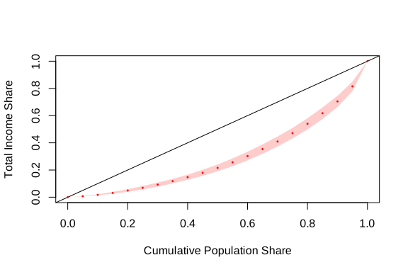
Figure 3.1: Estimated Lorenz curve for household income
The formula = ~Income argument specifies the income variable on which the cumulative distribution will be calculated. The argument design = gini_design indicates the previously defined sample design object, which contains the information related to weights, strata and clusters of the survey. For its part, quantiles = seq(0, 1,.05) defines the distribution points at which the Lorenz curve will be evaluated, generating percentiles from 0 to 1 in increments of 0.05. Finally, the alpha =.01 argument establishes a significance level of 1%, which is equivalent to constructing 99% confidence intervals for the estimates associated with the curve.
### Correlation estimation {#estimacion-de-la-correlacion}
In the study of household surveys, in addition to describing variables individually, it is essential to analyze how they relate to each other. One of the most used tools for this purpose is the Pearson correlation coefficient, which measures the strength and direction of the linear relationship between two numerical variables. This coefficient takes values between -1 and 1. A positive value indicates that both variables tend to increase simultaneously, while a negative value indicates that when one variable increases, the other tends to decrease. For their part, values close to zero suggest the absence of a strong linear relationship between the analyzed variables.
For example, in a household survey it may be of interest to study whether there is an association between household income and their level of expenditure, as well as evaluate the magnitude of said relationship. This type of analysis allows us to better understand the economic and social patterns observed in the population.
In complex surveys, it is necessary to incorporate sampling weights so that the estimate is representative of the population. This adjustment takes into account stratification, clustering, and unequal selection probabilities. The weighted calculation involves evaluating the covariance between the two variables and dividing it by the product of their weighted standard deviations, thus eliminating the influence of the measurement units. Assuming that \(\hat{\bar{x}}\) is an estimate of the population mean of the \(x\) variable, then the weight-adjusted Pearson correlation coefficient is expressed as: \[ \hat{\rho}_{xy} = \frac{\displaystyle \sum_{h} \sum_{i} \sum_{k} w_{hik} (y_{hik} - \hat{\bar{y}})(x_{hik} - \hat{\bar{x}})} {\sqrt{\displaystyle \sum_{h} \sum_{i} \sum_{k} w_{hik} (y_{hik} - \hat{\bar{y}})^2} \sqrt{\displaystyle \sum_{h} \sum_{i} \sum_{k} w_{hik} (x_{hik} - \hat{\bar{x}})^2}} \]
The survey package has the svyvar() function that allows obtaining weighted covariance matrices, from which the correlation can be calculated. Table 3.21 presents an example of estimation for the variance covariance matrix between household income and expenditure.
| Variable | Income | Expenditure | |
|---|---|---|---|
| Income | Income | 243719 | 98337 |
| Expenditure | Expenditure | 98337 | 77887 |
The svyvar function estimates the variance and covariance matrix considering the sample design. From this matrix the correlation can be obtained by applying the following instructions:
cov_xy <- cov_matrix[1, 2]
sd_x <- sqrt(cov_matrix[1, 1])
sd_y <- sqrt(cov_matrix[2, 2])

weighted_cor <- cov_xy / (sd_x * sd_y)
weighted_cor
## [1] 0.714If you also want to perform statistical inference on the correlation, for example obtaining standard errors or confidence intervals, you can use replication methods (bootstrap/jackknife) compatible with the survey package. Another option is to use the svycor function from the jtools package to directly estimate the correlation:
##             Income Expenditure
## Income        1.00        0.71
## Expenditure   0.71        1.00
3.2 Hypothesis testing
In the analysis of data from household surveys, it is not enough to study each variable in isolation, such as estimating the average income of men and women in a country. It is also essential to compare groups and evaluate whether the differences observed between them reflect real inequalities in the population or if they could be explained simply by sampling error. For example, a frequently asked question is whether there are statistically significant differences in median income between male-headed households and female-headed households. This type of analysis makes it possible to identify social and economic gaps, in addition to generating useful evidence for the design and evaluation of public policies.
To answer these types of questions, hypothesis tests are used, that is, statistical procedures that allow statements about population parameters to be contrasted using the information observed in the sample. In the context of household surveys, these tests must adequately incorporate the characteristics of the sampling design in order to guarantee valid inferences and reliable results.
Hypothesis testing is a fundamental tool for evaluating statements about population parameters based on the information observed in a sample. Generally speaking, any hypothesis test is based on the contrast between two opposing propositions: the null hypothesis, denoted by \(H_0\), and the alternative hypothesis, denoted by \(H_1\). In the most common case of a two-sided test, these hypotheses are expressed as: \[ \begin{cases} H_{0}: & \theta = \theta_0 \\ H_{1}: & \theta \neq \theta_0 \end{cases} \]
where \(\theta\) represents the population parameter of interest and \(\theta_0\) a reference value specified under the null hypothesis. Depending on the objective of the analysis, the alternative hypothesis can also be formulated unilaterally, for example, when you want to evaluate whether \(\theta > \theta_0\) or whether \(\theta < \theta_0\). The purpose of the test is to determine whether the evidence contained in the sample is strong enough to reject the null hypothesis in favor of the alternative hypothesis.
Suppose \(\bar{y}_1\) and \(\bar{y}_2\) represent the population means of a variable \(y\) in two different domains, for example, the mean income of male-headed households and the mean income of female-headed households. So, the parameter of interest then corresponds to the difference: \[ \Delta = \bar{y}_1 - \bar{y}_2 \]
Its sample estimator is defined as: \[ \hat{\Delta} = \hat{\bar{y}}_1 - \hat{\bar{y}}_2 \]
For which, its standard error is estimated by the following expression: \[ \widehat{se}(\hat{\Delta}) = \sqrt{ \widehat{Var}(\hat{\bar{y}}_1) + \widehat{Var}(\hat{\bar{y}}_2) - 2\widehat{Cov}(\hat{\bar{y}}_1, \hat{\bar{y}}_2) } \]
The presence of the covariance term is important because the estimates of both domains usually come from the same sample and, therefore, are not necessarily independent. Once the estimator and its standard error have been calculated, the hypothesis contrast is carried out using the following test statistic: \[ t = \frac{\hat{\Delta}} {\widehat{se}(\hat{\Delta})} \sim t_{df} \]
which approximately follows a Student \(t\) distribution with \((df)\) degrees of freedom. In practice, these degrees of freedom are usually approximated by \(df = n_I - H\), where \(n_I\) represents the number of primary sampling units and \(H\) the number of strata. Under the null hypothesis, high absolute values of the \(t\) statistic constitute evidence against \(H_0\). In a complementary manner, a confidence interval can also be constructed for the parameter \(\Delta\). For a confidence level of \((1-\alpha)100\%\), said interval is given by: \[ \hat{\Delta} \;\pm\; t_{(1-\alpha/2,df)} \, \hat{se}(\hat{\Delta}). \]
This interval provides a range of plausible values for the population difference and is a useful tool for evaluating both the magnitude and statistical significance of the observed differences between groups.
In R, these tests can be implemented using the svyttest() function of the survey package, which automatically incorporates the adjustments associated with the sample design. From the results presented in Table 3.22 it can be concluded that, with a confidence level of 95%, there is not sufficient statistical evidence to affirm that average incomes differ by sex.
| statistic | p_value | gl | ci_lower | ci_upper | estimated_difference |
|---|---|---|---|---|---|
| 1.36 | 0.176 | 118 | -12.8 | 69.4 | 28.3 |
Another hypothesis of interest consists of evaluating whether the average household income differs depending on the sex of the head within the urban area, as presented in Table 3.23. The results indicate that the null hypothesis \(H_0\) is not rejected, so there is not enough statistical evidence to affirm that average income differs by sex in the urban area.
urban_subset <- survey_design %>%
  filter(Zone == "Urban")

ttest_urban <- svyttest(Income ~ Sex, design = urban_subset, level = 0.95)| statistic | p_value | gl | ci_lower | ci_upper | estimated_difference |
|---|---|---|---|---|---|
| 1.57 | 0.122 | 63 | -12.3 | 102 | 44.7 |
The procedure described is not limited to means, but can also be applied to proportions, totals, ratios or any function differentiable from totals. In all cases, the contrast is based on the point estimate, its variance (including covariances when applicable) and the comparison with the \(t\) distribution adjusted to the sample design. ## Contrast estimation {#estimacion-de-contrastes}
In the analysis of household surveys it is common that the interest is not limited to comparing only two populations, but several simultaneously. For example, it may be necessary to compare the average household income between different regions, geographic areas or population groups, in order to identify differences and establish patterns of inequality between them. In these types of situations, the mean difference tests presented above are limited, since they are designed to only compare pairs of populations.
To address more general comparisons, contrasts are used, which constitute a flexible tool to evaluate linear combinations of population parameters. In general terms, a contrast is defined as: \[ f\left(\theta_1,\theta_2,\ldots,\theta_J\right) = \sum_{j=1}^{J} a_j \theta_j, \]
where the coefficients \(a_j\) are known constants and \(\theta_j\) represent the parameters of interest. This approach allows a wide variety of comparisons between groups to be formulated and evaluated, including differences between means, multiple comparisons, and more complex combinations of parameters.
In R, methodological procedures for implementing contrasts in complex sampling designs are available through the svycontrast() function of the survey package. For example, if you want to compare the average income of two particular subpopulations (the Northern and Southern regions) you can use the contrast \(\bar{y}_{Norte} - \bar{y}_{Sur}\). Since the sample covers five regions in total, the contrast must be constructed by assigning coefficients only to the regions involved in the comparison and leaving coefficients equal to zero for the other regions. In this way, the contrast is defined as:
\[
1\times\hat{\bar{y}}_{Norte}+\left(-1\right)\times\hat{\bar{y}}_{Sur}+0\times\hat{\bar{y}}_{Centro}+0\times\hat{\bar{y}}_{Occidente}+0\times\hat{\bar{y}}_{Oriente}.
\]
This expression indicates that the contrast corresponds to the difference between the estimated means of the North and South regions, while the other regions do not participate in the comparison. In matrix form, the contrast can be written as: \[ \left[1,\,-1,\,0,\,0,\,0\right] \times \left[\begin{array}{c} \hat{\bar{y}}_{Norte}\\ \hat{\bar{y}}_{Sur}\\ \hat{\bar{y}}_{Centro}\\ \hat{\bar{y}}_{Occidente}\\ \hat{\bar{y}}_{Oriente} \end{array}\right]. \]
Consequently, the contrast vector associated with this comparison is \(\left[1,\,-1,\,0,\,0,\,0\right]\), where the positive and negative coefficients indicate the populations to be compared and the zeros represent the populations excluded from the contrast. The first step is to calculate the estimated means for each region using group_by() and survey_mean(), as presented in Table 3.24. The visible results object is constructed with srvyr; Additionally, an auxiliary object with a covariance matrix is created for subsequent contrasts. As a result, the estimated averages of income by region are obtained.
region_mean <- survey_design %>%
  group_by(Region) %>%
  summarise(mean = survey_mean(Income,
                               na.rm = TRUE,
                               vartype = c("se", "ci")))

region_mean_contrast <- svyby(formula = ~Income,
                              by = ~Region,
                              design = survey_design,
                              FUN = svymean,
                              na.rm = TRUE,
                              covmat = TRUE,
vartype = c("se", "ci"))| Region | mean | mean_se | mean_low | mean_upp |
|---|---|---|---|---|
| Norte | 552 | 55.4 | 443 | 662 |
| Sur | 626 | 62.4 | 502 | 749 |
| Centro | 651 | 61.5 | 529 | 772 |
| Occidente | 517 | 46.2 | 425 | 609 |
| Oriente | 542 | 71.7 | 400 | 684 |
The svycontrast() function returns the estimated contrast and its standard error. The arguments of this function are the averages of the estimated revenues (stat) and the contrast constants (contrasts), as shown in Table 3.25.
contrast_region_ns <- svycontrast(
  stat = region_mean_contrast,
  contrasts = list(north_south_difference = c(1, -1, 0, 0, 0))
)| contrast | estimate | variance | standard_error |
|---|---|---|---|
| north_south_difference | -73.4 | 6959 | 83.4 |
Note that these same results could be obtained by explicitly carrying out the process of constructing the contrast estimator and its estimated variance. If only the estimated average incomes of the North and South regions are considered, their difference is:
## [1] -73.4The next step is to calculate the variance and covariance matrix and from there extract the variances and covariances of the North and South regions, presented in Table 3.26:
| Region | Norte | Sur | Centro | Occidente | Oriente |
|---|---|---|---|---|---|
| Norte | 3065 | 0 | 0 | 0 | 0 |
| Sur | 0 | 3894 | 0 | 0 | 0 |
| Centro | 0 | 0 | 3778 | 0 | 0 |
| Occidente | 0 | 0 | 0 | 2136 | 0 |
| Oriente | 0 | 0 | 0 | 0 | 5136 |
To calculate the standard error of the difference (contrast), the properties of the variance will be used, as follows: \[ \widehat{se}\left(\hat{\bar{y}}_{Norte}-\hat{\bar{y}}_{Sur}\right)=\sqrt{\widehat {Var}\left(\hat{\bar{y}}_{Norte}\right)+ \widehat{Var}\left(\hat{\bar{y}}_{Sur}\right)- 2\, \widehat{Cov}\left(\hat{\bar{y}}_{Norte},\hat{\bar{y}}_{Sur}\right)} \]
Therefore:
## [1] 78.2Which corresponds to the same result obtained previously with the svycontrast() function. In addition to comparing only two populations, contrasts allow several comparisons of interest to be evaluated simultaneously between different groups.
On the other hand, suppose you want to compare average incomes between different geographic regions. In particular, contrasts such as \(\bar{y}_{Norte} - \bar{y}_{Centro}\), \(\bar{y}_{Sur} - \bar{y}_{Centro}\) and \(\bar{y}_{Occidente} - \bar{y}_{Oriente}\) could be considered. Each of these expressions represents a specific linear contrast between regional means. Jointly, these contrasts can be organized using the following contrast matrix: \[ \left[\begin{array}{ccccc} 1 & 0 & -1 & 0 & 0\\ 0 & 1 & -1 & 0 & 0\\ 0 & 0 & 0 & 1 & -1 \end{array}\right] \]
In this matrix, each row defines a different contrast and each column corresponds to one of the regions considered in the analysis. The positive and negative coefficients indicate the means that participate in each comparison, while the zeros represent the regions that do not participate in the corresponding contrast. Below is the implementation of the contrasts in R, the results of which are presented in Table 3.27. From these results, it can be concluded that the Southern and Central regions have the most similar average household incomes, given that the estimated difference between both regions is the smallest among the contrasts evaluated.
contrast_regions <- svycontrast(
  stat = region_mean_contrast,
  contrasts = list(
    north_south = c(1, 0, -1, 0, 0),
    south_center = c(0, 1, -1, 0, 0),
    west_east = c(0, 0, 0, 1, -1)
  )
)| contrast | estimate | variance | standard_error |
|---|---|---|---|
| north_south | -98.4 | 6843 | 82.7 |
| south_center | -25.0 | 7673 | 87.6 |
| west_east | -24.7 | 7272 | 85.3 |
It is also possible to build contrasts between variables associated with different population groups, as occurs when comparing average income according to sex. Following the same procedure as the previous example, the first step is to estimate the average income for each group, in this case men and women, as presented in Table 3.28.
sex_mean <- survey_design %>%
  group_by(Sex) %>%
  summarise(mean = survey_mean(Income,
                               na.rm = TRUE,
                               vartype = c("se", "ci")))

sex_mean_contrast <- svyby(formula = ~Income,
                           by = ~Sex,
                           design = survey_design,
                           FUN = svymean,
                           na.rm = TRUE,
                           covmat = TRUE,
vartype = c("se", "ci"))| Sex | mean | mean_se | mean_low | mean_upp |
|---|---|---|---|---|
| Female | 558 | 25.8 | 506 | 609 |
| Male | 586 | 34.6 | 517 | 654 |
In this case, the contrast of interest is given by \(\bar{y}_{F} - \bar{y}_{M}\), which allows quantifying the difference between the average income of women and that of men. Next, using the function svycontrast() of the survey package, the contrast estimation is obtained, the results of which are presented in Table 3.29. From these results, it is concluded that, on average, men receive 28.3 monetary units more than women, with an estimated standard error of 19.8 monetary units.
contrast_sex <- svycontrast(
  stat = sex_mean_contrast,
  contrasts = list(sex_difference = c(1, -1))
)| contrast | estimate | variance | standard_error |
|---|---|---|---|
| sex_difference | -28.3 | 431 | 20.8 |
Since the contrasts correspond to linear functions of parameters, it is also possible to apply them to ratio estimators. An example of this is to compare the relationship between expenses and income according to sex. In this case, first the expense-income ratio is estimated for each group and subsequently the contrast between these ratios is constructed. Below are the computational codes used to perform this analysis, the results of which are shown in Table 3.30:
sex_ratio <- survey_design %>%
  group_by(Sex) %>%
  summarise(ratio = survey_ratio(Income,
                                 Expenditure,
                                 na.rm = TRUE,
                                 vartype = c("se", "ci")))

sex_ratio_contrast <- svyby(formula = ~Income,
                            by = ~Sex,
                            denominator = ~Expenditure,
                            design = survey_design,
                            FUN = svyratio,
                            na.rm = TRUE,
                            covmat = TRUE,
vartype = c("se", "ci"))| Sex | ratio | ratio_se | ratio_low | ratio_upp |
|---|---|---|---|---|
| Female | 1.52 | 0.046 | 1.43 | 1.61 |
| Male | 1.56 | 0.070 | 1.43 | 1.70 |
The svycontrast() function is not limited only to the comparison of means or totals, but also allows the construction of contrasts between other parameters of interest, such as ratios and proportions estimated from complex sampling designs. The computational codes used to perform this analysis are presented below, the results of which are shown in Table 3.31. From these results, it can be concluded that the difference between the estimated ratios is 0.045 in favor of men.
contrast_sex_ratio <- svycontrast(
  stat = sex_ratio_contrast,
  contrasts = list(sex_difference = c(1, -1))
)| contrast | estimate | standard_error | variance |
|---|---|---|---|
| sex_difference | -0.046 | 0.042 | 0.002 |
3.3 Visualization of continuous variables
The graphical representation of continuous variables is an essential component in the analysis of household surveys. Well-designed graphs allow you to identify distributions, trends and relationships between variables, facilitating the interpretation of the findings and their communication to different audiences (Wilkinson, 2005). A fundamental aspect in this context is that the graphs must incorporate the sampling weights to reflect the distribution of the population of interest.
This section uses the ggplot2 (Wickham, Chang, et al., 2026) and patchwork (Pedersen, 2025) packages for graph construction and composition, combined with survey (Lumley, 2024) and srvyr (Freedman Ellis & Schneider, 2024).
3.3.1 Histograms
A histogram is a graphical representation of the distribution of a continuous numerical variable, constructed from rectangles whose height is proportional to the frequency of observations within certain class intervals. In the context of household surveys, weighted histograms allow us to approximate the distribution of the variable in the population, incorporating the expansion factors associated with the sampling design.
Below is the weighted histogram of the variable Income, constructed incorporating the sampling weights (wk) in order to represent the estimated distribution of income in the population. The results obtained are shown in Figure 3.2:
weighted_income_hist <- ggplot(
  data = survey_data,
  aes(x = Income, weight = wk)) +
  geom_histogram(aes(y = ..density..)) +
  ylab("") +
  ggtitle("Weighted histogram")
weighted_income_hist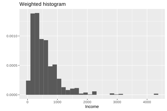
Figure 3.2: Weighted histogram of household income
In this code, the graph construction starts with the survey_data database. Within aes(), the argument x = Income indicates that the variable represented on the horizontal axis corresponds to income, while weight = wk incorporates the sampling weights to construct a weighted histogram that reflects the estimated distribution in the population. The function geom_histogram() generates the histogram, and using aes(y = ..density..), the height of the bars is expressed in terms of density rather than absolute frequencies. ylab("") then removes the vertical axis label, and ggtitle("Weighted histogram") adds a descriptive title to the chart.
Histograms also allow you to visually compare the distribution of a variable between different subgroups of the population using the argument fill, which assigns a different color to each category. For example, it is possible to compare the income distribution between urban and rural areas, as shown in Figure 3.3:
zone_colors <- c(Urban = "#48C9B0", Rural = "#117864")

weighted_zone_hist <- ggplot(survey_data, aes(x = Income, weight = wk)) +
  geom_histogram(
    aes(y = ..density.., fill = Zone),
    alpha = 0.5, position = "identity") +
  scale_fill_manual(values = zone_colors) +
  ylab("") +
  ggtitle("Weighted")

weighted_zone_hist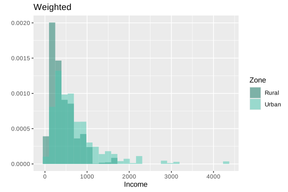
Figure 3.3: Weighted histogram of income by geographical area
In this code, a weighted histogram is constructed using the survey_data database, where x = Income defines the variable represented on the horizontal axis and weight = wk incorporates the sample weights to reflect the population distribution of income. The geom_histogram() function generates the histogram and, through aes(y =..density.., fill = Zone), represents the bars in terms of density and assigns different colors according to the Zone variable, allowing the income distribution to be visually compared between zones. The alpha = 0.5 argument adds transparency to the bars to make it easier to overlay histograms, while position = "identity" allows the distributions to be drawn on top of each other rather than stacked. Subsequently, scale_fill_manual(values = zone_colors) manually defines the colors associated with each zone. Finally, ylab("") removes the vertical axis label, ggtitle("Weighted") adds a title to the chart.
Additionally, it is possible to superimpose smoothed density curves using the geom_density() function, which allows the shape of the distribution of the analyzed variable to be continuously displayed. This type of representation facilitates the identification of patterns such as asymmetries, concentration of observations or the presence of multiple modes. An example of this type of graph is presented in Figure 3.4:
weighted_income_hist + geom_density(fill = "blue", alpha = 0.3) |
  weighted_zone_hist + geom_density(aes(fill = Zone), alpha = 0.3) +
  theme(legend.position = "top")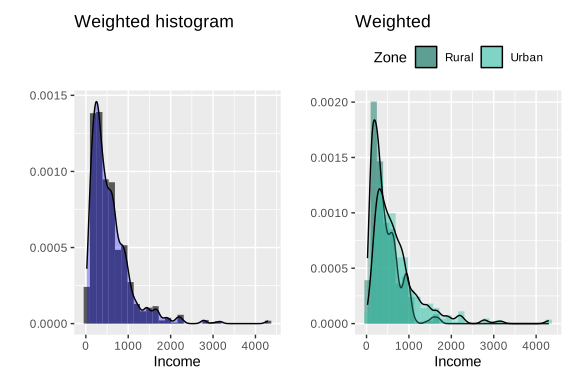
Figure 3.4: Histograms with superimposed density curves for income and expenditure
3.3.2 Box plots (boxplots)
Boxplots allow you to identify outliers and evaluate the dispersion of the distribution. Introduced by John Tukey in 1977, they are a graphic representation that summarizes the distribution of a variable using statistics based on quartiles, allowing the median, dispersion of the data and the presence of outliers to be identified. In the context of household surveys, this type of graph is useful for comparing distributions between different population groups in a compact and visually intuitive way.
To construct boxplots weighted in ggplot2 the function geom_boxplot() is used, as shown in Figure 3.5. In this case, the function ggplot() starts the construction of the graph using the survey_data database, where x = Income defines the numerical variable analyzed and weight = wk incorporates the sampling weights to represent the estimated distribution in the population. Subsequently, geom_boxplot() generates the box plots and, using aes(fill = Zone) or aes(fill = Sex), assigns different colors to each category of the variables Zone and Sex, respectively, facilitating visual comparison between groups. The coord_flip() function inverts the axes to present the boxplots horizontally, thus improving their readability. For its part, scale_fill_manual() allows you to manually define the colors associated with each category using the zone_colors and sex_colors vectors.
weighted_zone_boxplot <- ggplot(survey_data, aes(x = Income, weight = wk)) +
  geom_boxplot(aes(fill = Zone)) +
  ggtitle("Weighted") +
  coord_flip() +
  scale_fill_manual(values = zone_colors)

sex_colors <- c(Male = "#5DADE2", Female = "#2874A6")

weighted_sex_boxplot <- ggplot(survey_data, aes(x = Income, weight = wk)) +
  geom_boxplot(aes(fill = Sex)) +
  ggtitle("Weighted") +
  coord_flip() +
  scale_fill_manual(values = sex_colors)

weighted_zone_boxplot | weighted_sex_boxplot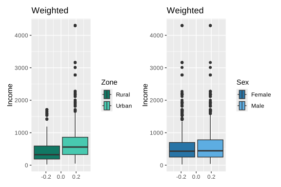
Figure 3.5: Weighted boxplots of income by area and sex
In addition to the tools available in ggplot2, the survey package offers specialized functions such as svyhist() and svyboxplot(), which directly incorporate the features of complex sample design into the construction of the graphs. These functions allow us to obtain graphical representations consistent with the survey design, facilitating the exploratory analysis of the numerical variables. An example of its application is presented in Figure 3.6.
par(mfrow = c(1, 2))
svyhist(~Income, survey_design,
  main = "Household income",
  col  = "grey80", xlab = "Income",
  probability = FALSE)

svyboxplot(Income ~ Zone, survey_design,
  col  = "grey80",
  ylab = "Income", xlab = "Zone")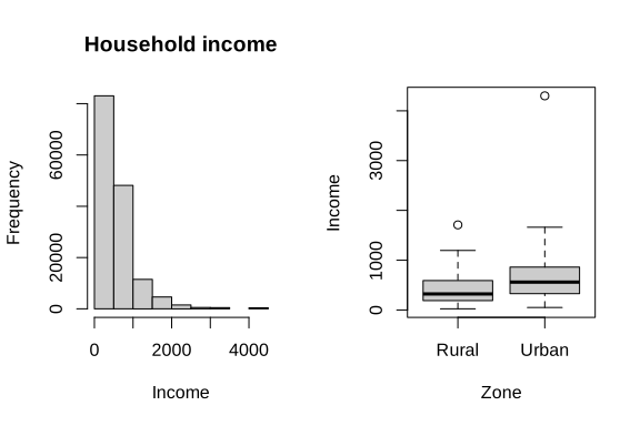
Figure 3.6: Histogram and boxplot of income adjusted to the complex sample design
3.3.3 Scatter plots
Scatter plots allow you to visually explore the relationship between two continuous variables, facilitating the identification of patterns of association, trends, and possible outliers. In the context of surveys with complex sample designs, it is important to incorporate information on sampling weights so that the graphical representation adequately reflects the relative contribution of each observation in the population.
According to Lumley (2010), when working with large data sets, plotting all points simultaneously can result in graphs that are difficult to interpret due to overlapping observations. However, in moderately sized samples, a simple and effective strategy is to represent the weights by the size of the symbols in the scatterplot. In this way, the observations with the greatest population weight appear visually highlighted. An example of this type of representation is presented in Figure 3.7:
weighted_basic_scatter <- ggplot(
  data = survey_data,
  aes(y = Income, x = Expenditure)) +
  geom_point(aes(size = wk), alpha = 0.3)

weighted_basic_scatter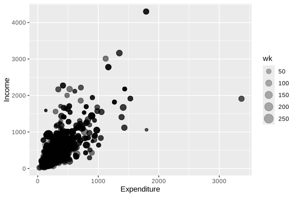
Figure 3.7: Scatter diagram between household income and expenditure
In this code, a scatterplot is constructed between the variables x = Expenditure and y = Income. The geom_point() function adds the points on the graph and, using aes(size = wk), uses the sampling weights (wk) to control the size of each point, so that observations with greater population representation appear visually more prominent. The alpha = 0.3 argument incorporates transparency to the points, reducing the overlapping problem and facilitating the visualization of areas with a high concentration of observations.
Additionally, it is possible to incorporate grouping variables in the scatter diagrams using the arguments shape and color, which allow observations to be visually differentiated according to specific categories of the population. This facilitates the identification of differentiated patterns between groups and improves the interpretation of the relationship between the analyzed variables. An example of this type of representation is presented in Figure 3.8.
weighted_zone_scatter <- ggplot(
  data = survey_data,
  aes(y = Income, x = Expenditure, shape = Zone)) +
  geom_point(aes(size = wk, color = Zone), alpha = 0.3) +
  labs(size = "Weight") +
  scale_color_manual(values = zone_colors)

weighted_zone_scatter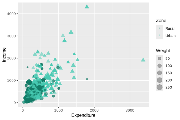
Figure 3.8: Scatter diagram between income and expenditure by geographic area