Chapter 5 Regression models
Regression models are one of the most widely used tools for analyzing survey data, since they make it possible to study the relationship between a variable of interest and a set of explanatory variables. Through these models, it is possible to assess how certain population characteristics vary according to demographic, social, or economic factors observed in the sample. However, the validity of the results obtained depends on appropriate model specification and on correctly accounting for the characteristics of the survey sampling design.
In general terms, regression models seek to describe and quantify the association between a response (dependent) variable and one or more explanatory (independent) variables, providing elements for statistical interpretation and for drawing inferences about the study population. Nevertheless, the validity of the results obtained depends, to a large extent, on appropriate model specification and on correctly accounting for the characteristics of the survey sampling design (Heeringa et al., 2017).
For example, household income can be analyzed as a response variable as a function of characteristics such as educational attainment and the employment status of household members, considered as explanatory variables. Using information from household surveys, this type of model makes it possible to identify patterns of association, quantify the effect of different socioeconomic factors on income, and generate empirical evidence useful for the design, monitoring, and evaluation of public policies.
However, because household surveys are based on complex sampling designs, classical regression methods, developed under simple random sampling assumptions, may be inappropriate. Ignoring the characteristics of the sampling design can generate biased estimates of regression coefficients, as well as underestimation of their standard errors and variances, compromising the validity of statistical inferences.
Consequently, the analysis of survey data requires close attention to the sampling design. Incorporating survey weights and the adjustments corresponding to stratification and clustering makes it possible to obtain valid and precise inferences. In addition, simplified alternatives have been proposed in some cases, such as the use of normalized weights or approximate weighting approaches, which seek to balance methodological complexity with the practical feasibility of the analysis.
The study of regression under complex sampling designs has a well-documented history. Kish & Frankel (1974) were among the first to discuss the impact of these designs on inferences derived from regression models. Subsequently, Fuller (1975) developed a variance estimator based on linearization techniques for multiple linear regression models with unequal weighting, and introduced specific methods for stratified and two-stage designs.
Later, Shah et al. (1977) addressed the problem of violations of classical assumptions when working with survey data, proposing robust inference alternatives for the parameters. In parallel, Binder (1983) focused on the sampling distributions of regression estimators in finite populations, establishing procedures for estimating variances under complex schemes.
In the following years, Skinner et al. (1989) expanded these contributions through variance estimators for regression coefficients that incorporated stratification and clustering, explicitly recommending the use of linearization methods or alternative techniques for variance estimation. Later, Fuller (2002) provided a compendium of estimation methods applicable to regression models in complex surveys, while Pfeffermann (2011) discussed more recent developments, such as q-weighted weighting methods, presenting empirical evidence of their usefulness.
5.1 Model formulation
Regression models under complex sampling designs make it possible to move beyond descriptive statistics and approach causal or predictive explanations, provided that the particularities of the sampling design are recognized and adjusted for. Their correct application opens the possibility of examining how sociodemographic and economic characteristics are associated with different outcomes of interest, contributing key evidence for public policy formulation.
As a starting point, it is useful to present the general structure of regression models. The most basic formulation corresponds to the simple linear regression model, which describes the relationship between a response variable and a single explanatory variable through the following expression:
\[ y = \beta_{0} + \beta_{1}x + \varepsilon \]
Here, \(y\) represents the response (dependent) variable, \(x\) the explanatory (independent) variable, \(\beta_{0}\) the model intercept, \(\beta_{1}\) the coefficient associated with the independent variable, and \(\varepsilon\) the error term, which captures the variability not explained by the model and can be interpreted as the difference between the observed value and the value estimated by the model, denoted by \(\hat{y}_k\).
In many empirical applications, and especially in the analysis of household surveys, the phenomenon of interest depends simultaneously on multiple factors. In these cases, multiple linear regression models are used, incorporating several explanatory variables:
\[ y = \beta_{0} + \beta_{1}x_{1} + \cdots + \beta_{p}x_{p} + \varepsilon, \]
where each coefficient \(\beta_{j}\) quantifies the association between the response variable and the corresponding covariate \(x_{j}\), holding the other variables included in the model constant. More compactly, the model can be expressed using matrix notation as:
\[ y_{k} = \mathbf{x}_{k}\boldsymbol{\beta} + \varepsilon_{k}, \quad k=1,\ldots,n, \]
where \(\mathbf{x}_{k} = [1, x_{1i}, \ldots, x_{pi}]\) represents the vector of covariates associated with unit \(k\), while \(\boldsymbol{\beta} = [\beta_{0}, \beta_{1}, \ldots, \beta_{p}]'\) corresponds to the vector of unknown model parameters. In this context, the expected value of the response variable conditional on the set of covariates can be expressed as:
\[ E(y \mid \mathbf{x}) = {\beta}_{0} + {\beta}_{1}x_{1} + \cdots + {\beta}_{p}x_{p} \]
Linear regression models are based on a series of theoretical assumptions that guarantee the validity of the estimates and the inferences derived from the model. First, it is assumed that the expected value of the residuals conditional on the covariates is equal to zero, that is, \(E(\varepsilon_{k} \mid \mathbf{x}_{k}) = 0\), which implies the absence of systematic bias in the estimation of the response variable. Likewise, homogeneity of the error variance is assumed, so that residual variability remains constant for all values of the covariates, that is, \(Var(\varepsilon_{k} \mid \mathbf{x}_{k}) = \sigma^2\). In addition, the errors are considered to follow a normal distribution with zero mean and constant variance, expressed as \(\varepsilon_{k} \mid \mathbf{x}_{k} \sim N(0,\sigma^2)\), and the residuals associated with different observations are assumed to be independent of one another, such that \(Cov(\varepsilon_{k},\varepsilon_{j}\mid \mathbf{x}_{k},\mathbf{x}_{j})=0\).
The validity of linear regression models depends on the fulfillment of several classical assumptions widely discussed in the specialized literature. Taken together, these assumptions allow the estimators obtained through the model to have desirable statistical properties, such as unbiasedness, efficiency, and consistency.
5.2 Use of sampling weights
When working with data from surveys based on complex sampling designs, the classical assumptions of regression models are rarely strictly satisfied, since observations do not come from simple and independent random samples, but from selection schemes that incorporate elements such as stratification, clustering, and unequal probabilities of selection. For example, the presence of clustering may violate the assumption of independence of errors, since individuals belonging to the same household, segment, or geographic area tend to share similar characteristics. Similarly, unequal probabilities of selection and weighting adjustments can generate heterogeneity in the variance of observations, violating the assumption of homoscedasticity.
In this context, a fundamental question arises: how should sampling weights be incorporated into regression models? The answer is not straightforward, since survey weights reflect not only probabilities of selection, but also various adjustments associated with nonresponse, calibration, and coverage corrections. Although their use makes it possible to produce estimates that are representative of the population, the direct incorporation of weights into models can also reduce statistical efficiency and increase estimator variability.
In general terms, the literature distinguishes two main approaches to this problem (Heeringa et al., 2017). The first corresponds to the design-based approach, whose objective is to obtain valid inferences for the target population while respecting the characteristics of the sample selection process. From this perspective, sampling weights are essential for correcting unequal probabilities of inclusion and producing unbiased estimates of the regression coefficients. However, this approach does not protect against possible model specification errors; that is, even when the estimates are valid from a design perspective, the model may not adequately represent the relationships existing in the population.
The second corresponds to the model-oriented approach, according to which weights are not necessarily required as long as the model is correctly specified and the sampling mechanism is non-informative. Under this assumption, the relationships between the variables observed in the sample coincide with those in the population, so the sampling design does not introduce relevant biases in parameter estimation. From this perspective, incorporating weights could even be counterproductive, by unnecessarily increasing the variance of the estimators and, consequently, the standard errors.
The discussion about whether to use weights in regression models has been extensively developed in the specialized literature, particularly in works such as Skinner et al. (1989) and Pfeffermann (2011). In practice, a frequent methodological recommendation is to estimate models both with and without weights and then compare the results obtained. If including the weights produces important changes in the estimated coefficients or modifies the substantive conclusions of the analysis, this suggests that the sampling design is informative or that the model has specification problems, making the use of weights advisable (United Nations Statistics Division, 2026). Conversely, if the coefficients remain relatively stable and the weights only increase the standard errors, it may be considered that the model adequately captures the structure of the data and that the use of weights is not strictly necessary.
In applied terms, this decision usually depends on the analytical purpose of the study. When the objective is to carry out descriptive inference and produce estimates that are representative of the population, the use of weights is indispensable. By contrast, in contexts of analytical inference oriented toward the study of associations, causal relationships, or hypothesis tests, both weighted and unweighted models may be used, especially when the model incorporates variables related to the sampling design, such as strata or clusters. Nevertheless, the use of unweighted models must be carefully justified, since it implies assuming more restrictive conditions about the sample selection mechanism and the correct specification of the statistical model.
In summary, when weighting is chosen, weights correct possible biases from over- or underrepresentation of certain groups and help obtain more accurate variance estimates. Within the design-based approach, this allows the results to approximate unbiased values comparable to those that would be obtained in a complete census, even when the model is not optimally formulated. However, when weights are highly dispersed, they can increase the variance of the estimated parameters and make the estimates unstable, which is why in explanatory or analytical contexts unweighted models may, at times, yield more consistent and efficient results.
In any case, if the model is misspecified, ignoring sampling weights can lead to biased, uninformative estimates, or even estimates lacking inferential validity. For this reason, the appropriate selection of the variables included in the model is a fundamental aspect of the analysis. To address these issues, various adjustment strategies have been proposed to achieve a balance between both objectives. The most commonly used procedures include the following:
Senate-type weights: this procedure adjusts the weights so that their sum matches the sample size rather than the population size. The objective is to maintain the relative representativeness of the units while reducing the dispersion of the original weights, which is particularly advantageous in surveys where there is high variability among expansion factors. Thus, the new weights are \(w_k^{Senate} = w_k \times \frac{n}{\sum w_k}\).
Normalized weights: in this approach, the original weights are rescaled so that their sum is equal to one, which avoids an unnecessary increase in variance in the models. This technique is especially useful when working with different data subsets (for example, models estimated in subpopulations) or when seeking to minimize variance inflation. Thus, the new weights are \(w_k^{Normalized} = \frac{w_k}{\sum w_k}\).
It is important to note that, in both methods, the adjusted weights are obtained through direct multiplicative transformations of the original sampling weights. Therefore, they should not be used to calculate population sizes or totals. Likewise, these procedures do not alter estimates of ratios, such as means or proportions, since in those cases the weights cancel out in the quotient. In practice, the use of these adjustments can be considered a pragmatic solution in contexts where specialized survey software is not available. However, when tools such as the R packages survey (Lumley, 2024) and srvyr (Freedman Ellis & Schneider, 2024), described in previous chapters, are available, rescaling is no longer necessary, since these packages apply the appropriate treatment to preserve both representativeness and the inferential properties of the model.
5.3 Estimation of model parameters
For fitting regression models with household surveys, advanced inferential methodologies have been developed that integrate sources of uncertainty within a single analytical framework, seeking to reflect both the structure of the design and the assumptions and limitations of the model. Among the most relevant approaches are pseudo-likelihood (Molina & Skinner, 1992) and combined inference (Binder, 2011).
The pseudo-likelihood method extends traditional maximum likelihood techniques to adapt them to the particularities of complex sampling designs. In this approach, the sampling distribution defined by the design plays a central role, while the model distribution moves into the background. Although in contexts of well-specified models pseudo-likelihood-based estimators tend to be unbiased or consistent, their main virtue lies in avoiding the biases that would arise from ignoring the sampling design. In practical terms, this method translates the traditional model into one that respects the way in which the data were obtained, ensuring more robust inferences.
By contrast, combined inference proposes a unified framework in which sampling variability and model uncertainty are integrated simultaneously. By considering both sources, this approach offers a more complete view of total variability and makes it possible to obtain more precise and reliable estimates. Its main contribution lies in avoiding the biases that can arise when the analysis is carried out exclusively from either the design or the model perspective. Thus, combined inference is especially useful in applications where population representativeness and the statistical robustness of the fitted models must be balanced.
When estimating the parameters of a linear regression model from a sample with a complex design, the standard approach changes. Consequently, traditional estimators, such as those obtained by maximum likelihood or least squares, may be biased and produce unreliable standard errors. In response to this situation, Wolter & Wolter (2007) proposes the use of robust nonparametric methods, such as Taylor linearization or bootstrap, to estimate variances and obtain valid inferences.
In the case of a simple linear regression model, the estimation of \(\beta_1\) under a complex sampling scheme is carried out using a weighted estimator, which can be expressed as follows:
\[ \hat{\beta_{1}} = \frac{\sum_{h} \sum_{i} \sum_{k} w_{hik}\,(y_{hik}-\hat{\bar{y}})(x_{hik}-\hat{\bar{x}})} {\sum_{h} \sum_{i} \sum_{k} w_{hik}\,(x_{hik}-\hat{\bar{x}})^{2}} = \frac{\hat{t}_{xy}}{\hat{t}_{xx}} \]
Here, \(\hat{\bar{y}}=\hat{t}_y/\hat{N}\) and \(\hat{\bar{x}}=\hat{t}_x/\hat{N}\) correspond to the estimated means of the study and auxiliary variables, respectively, while \(w_{hik}\) represents the sampling weights associated with each observation unit. This formulation explicitly incorporates these weights, making it possible to account for unequal probabilities of selection and the specific characteristics of the sampling design. Likewise, the estimated variance of \(\hat{\beta}_1\) can be approximated as:
\[ \widehat{Var}\left(\hat{\beta_{1}}\right) \approx \frac{\widehat{Var}(\hat{t}_{xy})+\hat{\beta}_{1}^{2}\widehat{Var}(\hat{t}_{xx})-2\hat{\beta}_{1}\widehat{Cov}(\hat{t}_{xy},\hat{t}_{xx})}{(\hat{t}_{xx})^{2}} \]
If \(\hat{\beta}_{1}\) corresponds to the slope estimator in a weighted simple linear regression model, then the intercept estimator \(\hat{\beta}_{0}\) is given by
\[ \hat{\beta}_{0} = \hat{\bar{y}} - \hat{\beta}_{1}\hat{\bar{x}} \]
Note that the variance of \(\hat{\beta}_{0}\) depends simultaneously on the estimators \(\hat{\bar{y}}\), \(\hat{\bar{x}}\), and \(\hat{\beta}_{1}\). For this reason, its approximation can be obtained using the properties of the variance of linear combinations of estimators, together with Taylor linearization techniques. From this procedure, the variance-covariance matrix of the model coefficients is derived, from which both the standard errors and the covariances associated with the parameter estimates are obtained.
In the case of multiple regression, if \(\hat{\boldsymbol{\beta}}\) represents the estimator of \(\boldsymbol{\beta}\), then the variance of each coefficient is estimated by considering its interdependence with the other parameters, which is reflected in the construction of a variance-covariance matrix that captures both individual variability and the covariances among all estimators. According to Kish & Frankel (1974), this calculation requires using weighted totals of squares and cross-products for all combinations between the dependent variable \(y\) and the set of predictors \(\mathbf{x} = (1, x_1, \ldots, x_p)\). In general terms:
\[ \widehat{Var}(\hat{\boldsymbol{\beta}}) = \hat{\boldsymbol\Sigma} = \begin{bmatrix} \widehat{Var}(\hat{\beta}_{0}) & \widehat{Cov}(\hat{\beta}_{0},\hat{\beta}_{1}) & \cdots & \widehat{Cov}(\hat{\beta}_{0},\hat{\beta}_{p}) \\ \widehat{Cov}(\hat{\beta}_{0},\hat{\beta}_{1}) & \widehat{Var}(\hat{\beta}_{1}) & \cdots & \widehat{Cov}(\hat{\beta}_{1},\hat{\beta}_{p}) \\ \vdots & \vdots & \ddots & \vdots \\ \widehat{Cov}(\hat{\beta}_{0},\hat{\beta}_{p}) & \widehat{Cov}(\hat{\beta}_{1},\hat{\beta}_{p}) & \cdots & \widehat{Var}(\hat{\beta}_{p}) \end{bmatrix} \]
This chapter shows how to implement these models in R using the survey package (Lumley, 2024), together with srvyr (Freedman Ellis & Schneider, 2024) and tidyverse (Wickham, Averick, et al., 2026) to organize the workflow. It covers specification of the sampling design, estimation of linear and logistic models, and the calculation of standard errors and design-adjusted hypothesis tests, integrating theoretical foundations with reproducible practical examples. To illustrate the concepts developed up to this point, the same database used throughout the book will be used. The process begins by loading the packages, the data, and defining the sampling design:
library(survey)
library(srvyr)
library(tidyverse)

data(BigCity, package = "TeachingSampling")
survey_data <- readRDS("Data/encuesta.rds")

survey_design <- survey_data %>%
  as_survey_design(
    strata = Stratum,
    ids = PSU,
    weights = wk,
    nest = TRUE
  )
The examples developed throughout this chapter will use the same subgroups considered in the previous chapters.
urban_subset <- survey_design %>%
  filter(Zone == "Urban")

rural_subset <- survey_design %>%
  filter(Zone == "Rural")

female_subset <- survey_design %>%
  filter(Sex == "Female")

male_subset <- survey_design %>%
  filter(Sex == "Male")
In order to fit a regression model between the income and expenditure variables, it is useful first to explore the relationship between them. For this purpose, a scatter plot is constructed with ggplot2, which makes it possible to visually assess the shape and strength of the association. The result is presented in Figure 5.1.
unweighted_plot <- ggplot(
  data = survey_data,
  aes(x = Expenditure, y = Income)
) +
  geom_point() +
  geom_smooth(method = "lm", se = FALSE)

unweighted_plot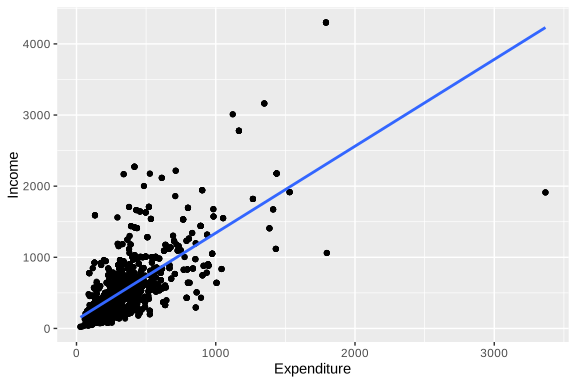
Figure 5.1: Scatter plot between expenditure and income in the sample (unweighted)
The sample data preserve an approximately linear relationship between income and expenditure, although greater dispersion is observed among the values corresponding to households with higher expenditure levels. Once the graphical exploration of the data has been completed, the linear regression models are fitted.
To fit models incorporating the expansion factors, the svyglm function from the survey package is used; this function makes it possible to estimate linear models while explicitly incorporating the characteristics of the sampling design. In this case, the expression Income ~ Expenditure specifies that the variable Income is modeled as a function of the variable Expenditure; that is, a simple linear regression is fitted in which expenditure acts as the explanatory variable for income. The argument design = survey_design indicates that the model must use the previously defined sampling design object, while family = stats::gaussian() specifies that a linear model with a normal distribution is fitted, equivalent to a classical linear regression.
fit_svy <- svyglm(
  Income ~ Expenditure + Zone + Sex,
  design = survey_design,
  family = stats::gaussian()
)

fit_svy
## Stratified 1 - level Cluster Sampling design (with replacement)
## With (238) clusters.
## Called via srvyr
## Sampling variables:
## - ids: PSU
## - strata: Stratum
## - weights: wk
##
## Call: svyglm(formula = Income ~ Expenditure + Zone + Sex, design = survey_design,
## family = stats::gaussian())
##
## Coefficients:
## (Intercept) Expenditure ZoneUrban SexMale
## 73.58 1.22 66.65 20.64
##
## Degrees of Freedom: 2604 Total (i.e. Null); 116 Residual
## Null Deviance: 635000000
## Residual Deviance: 309000000 AIC: 38300The output above corresponds to the fit of a linear regression model in which the variable Income is explained by the variables Expenditure, Zone, and Sex. The results indicate the existence of a positive relationship between income and expenditure, such that, holding the other variables constant, expected income increases by approximately 1.22 units for each additional unit of expenditure.
Likewise, systematic differences associated with the sociodemographic characteristics included in the model are evident: residing in an urban area is associated with an average increase of 66.65 units in income relative to the reference category, while being male is associated with an increase of 20.64 units compared with the base sex category. The estimated intercept, equal to 73.58, represents the expected income level for the model reference category (rural area and female sex) when expenditure is equal to zero.
5.4 Model diagnostics
In the analysis of household surveys, the evaluation of a statistical model is an important aspect that guarantees the validity of the inferences. The literature notes that an appropriately specified model depends not only on the selection of covariates, but also on the fulfillment of the assumptions that support the consistency and reliability of the results (Tellez Piñerez & Lemus Polanía, 2015).
For linear regression models applied to complex surveys, it is necessary to examine different aspects related to goodness of fit and the behavior of the errors. As indicated above, these include the explanatory capacity of the model, the normality and homogeneity of the residual variance, the independence of errors, and the possible presence of influential observations or outliers that may affect the estimates.
These checks are particularly important in the context of complex sampling designs, where characteristics such as stratification, clustering, and the use of expansion factors can intensify problems associated with heteroscedasticity, dependence among observations, or sensitivity to extreme values. For this reason, model diagnostics should not be limited to the classical assumptions of regression, but should also incorporate the particularities derived from the survey design. The systematic application of these procedures makes it possible to assess the robustness of the model, strengthen confidence in the inferences, and ensure that the results obtained are representative and useful for both applied social research and public policy analysis.
5.4.1 Coefficient of determination
One of the most widely used measures for evaluating the fit of a regression model is the coefficient of determination, denoted by \(R^{2}\) and also known as the multiple correlation coefficient. This indicator quantifies the proportion of the variability of the dependent variable that is explained by the model. Its values range from zero to one: the closer it is to one, the greater the explanatory capacity of the model; by contrast, values close to zero indicate a low level of explanation of the observed variability. The magnitude of \(R^{2}\) should not be evaluated in absolute terms, but rather in light of the phenomenon being studied and the type of information available.
The coefficient is calculated from the total and error sums of squares, as \(R^{2} = 1 - \frac{SSE}{SST}\), where \(SST\) represents the total sum of squares and \(SSE\) the sum of squared errors. In surveys with complex sampling designs, this measure must be adjusted to incorporate the design structure and the sampling weights. The weighted estimator of the coefficient of determination is defined as:
\[ \hat{R}^2 = 1 - \frac{\widehat{SSE}}{\widehat{SST}} \]
where \(\widehat{SSE}\) is the weighted sum of squared errors, calculated as \(\widehat{SSE} = \sum_{h} \sum_{i} \sum_{k} w_{hik} \,(y_{hik} - x_{hik}\hat{\boldsymbol{\beta}})^2\); while \(\widehat{SST}\) represents the weighted total sum of squares, defined by \(\widehat{SST} = \sum_{h} \sum_{i} \sum_{k} w_{hik}\,(y_{hik} - \hat{\bar{y}})^2\).
Since \(R^{2}\) tends to increase as more variables are incorporated into the model, it is recommended to complement its interpretation with the adjusted coefficient of determination (\(R_{adj}^{2}\)), which introduces a penalty based on the number of covariates included and the sample size (Pfeffermann, 2011). This coefficient is defined as \(\hat{R}^2_{adj} = 1 - \frac{(n-1)}{(n-p)}(1 - \hat{R}^2)\), where \(n\) corresponds to the number of observations, \(p\) represents the number of estimated parameters, and \(\hat{R}^{2}\) denotes the weighted coefficient of determination defined above.
In this way, the adjustment makes it possible to evaluate the explanatory capacity of the model while controlling for the effect derived from incorporating new variables. This adjustment facilitates a more equitable comparison between models with different numbers of predictors and is particularly useful in survey analysis, where design complexity and the use of weights can have a notable influence on the magnitude of \(R^{2}\).
In R, the coefficient of determination \(R^{2}\) can be estimated from the previously fitted models. To do this, a null model is first fitted (including only the intercept), which makes it possible to calculate the weighted total sum of squares (\(\widehat{SST}\)).
null_model <- svyglm(Income ~ 1, design = survey_design)

s1 <- summary(fit_svy)
s0 <- summary(null_model)

wsst <- s0$dispersion[1]
wsse <- s1$dispersion[1]
The estimate of the coefficient of determination and its adjusted counterpart is obtained from the following calculation:
n <- nrow(survey_design)
p <- 4
r2 <- 1 - wsse / wsst
r2_adj <- 1 - ((n - 1) / (n - p)) * (1 - r2)

r2
## [1] 0.5138## [1] 0.51335.4.2 Residuals
In model diagnostics, residual analysis is one of the most relevant tools. If the model is correctly specified, the residuals act as an approximation of the unobserved errors and make it possible to assess indirectly whether the model assumptions are reasonably satisfied in the data. Their systematic review makes it possible to identify possible deviations in the specification, helping to determine whether the fit is adequate or whether, on the contrary, it is necessary to reconsider the functional form of the model or the estimation method used.
In surveys with complex sampling designs, Pearson residuals are a common tool for evaluating discrepancies between observed values and expected values under the fitted model. Following Heeringa et al. (2017), they are defined as:
\[ r_{k} = \frac{y_k - \mu_k}{\sqrt{\widehat{Var}(\mu_k)/w_k}}, \]
where \(\hat{\mu}_{k} = \mathbf{x}_{k}^{\top}\hat{\boldsymbol{\beta}}\) represents the expected value of \(y_{k}\) under the fitted model, \(w_{k}\) corresponds to the sampling weight associated with unit \(k\), and \(\widehat{Var}(\hat{\mu}_{k})\) denotes the estimated variance under the model family.
Pearson residuals are also used to evaluate key aspects of model fit, particularly the normality and homogeneity of the error variance. As a complement, the plot of residuals against fitted values is an especially informative diagnostic tool, since visual inspection makes it possible to detect possible systematic patterns suggesting violations of the assumptions of independence or heteroscedasticity.
The assumption of normality of the errors should also be checked explicitly. A standard tool for this purpose is the quantile-quantile plot (QQ plot), which compares the quantiles of the observed residuals with the theoretical quantiles of a normal distribution with the same mean and variance. An approximate alignment of the points along the 45° line indicates that the normality assumption is reasonable within the context of the model.
These diagnostics are applied below to the previously fitted models. For this purpose, the svydiags package (Valliant, 2024) is used; it was developed as an extension of the survey package for diagnosing models estimated under complex sampling designs. This package makes it possible to obtain standardized residuals directly, facilitating the evaluation of model assumptions in this type of context:
library(svydiags)
stdresids <- as.numeric(svystdres(fit_svy)$stdresids)
survey_design$variables <- survey_design$variables %>%
  mutate(stdresids = stdresids)
The normality analysis can be complemented with the histogram of standardized residuals, presented in Figure 5.2. The histogram of standardized residuals reveals a significant lack of fit with respect to the theoretical normal distribution curve (in red), which corroborates a violation of the normality assumption. The distribution of the residuals (shown in blue) has a much sharper and narrower peak than the normal curve, as well as marked positive skewness with an extended right tail. This discrepancy indicates that the model fails to capture the real variability of the data, suggesting the need to apply a transformation of the dependent variable or to use a model with a more flexible and robust distribution family.
ggplot(
  data = survey_design$variables,
  aes(x = stdresids)
) +
  geom_histogram(
    aes(y = ..density..),
    colour = "black",
    fill = "blue",
    alpha = 0.3
  ) +
  geom_density(size = 1, colour = "blue") +
  geom_function(fun = dnorm, colour = "red", size = 1) +
  labs(y = "")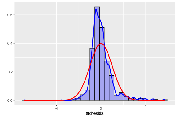
Figure 5.2: Histogram of standardized residuals with estimated density curve and theoretical normal distribution
Homoscedasticity of the errors (constant variance) is one of the central assumptions in regression models. Violating this assumption affects the efficiency of the model estimators. Since residuals represent the discrepancies between the observed values and the values fitted by the model, analyzing them as a function of predicted values or covariates is a fundamental diagnostic tool. Under an appropriately specified model, the residuals are expected to be randomly distributed around zero, without structured patterns; by contrast, the appearance of systematic shapes (such as funnel structures or curvatures) suggests the presence of heteroscedasticity (nonconstant variance) or possible functional relationships not captured by the model specification.
To evaluate this assumption, it is recommended to analyze the residuals graphically as a function of the estimated values \(\hat{\mu}_{k}\) or of specific covariates in the model. The appearance of systematic patterns in these plots constitutes evidence of heteroscedasticity or possible functional specification problems. In particular, to evaluate homoscedasticity with respect to the covariates included in the model, plots of residuals against each covariate are constructed and combined with patchwork (Pedersen, 2025).
library(patchwork)

g1 <- ggplot(
  data = survey_design$variables,
  aes(x = Expenditure, y = stdresids)
) +
  geom_point() +
  geom_hline(yintercept = 0)

g2 <- ggplot(
  data = survey_design$variables,
  aes(x = Zone, y = stdresids)
) +
  geom_point() +
  geom_hline(yintercept = 0)

g3 <- ggplot(
  data = survey_design$variables,
  aes(x = Sex, y = stdresids)
) +
  geom_point() +
  geom_hline(yintercept = 0)

(g1 | g2 | g3)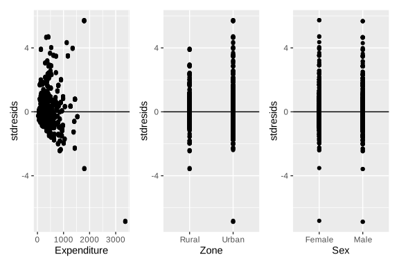
Figure 5.3: Plots of standardized residuals against each model covariate
Figure 5.3 presents the scatter plots of standardized residuals against the model covariates. Taken together, these results suggest possible limitations in the functional specification. In particular, for Expenditure, a slight curvature is observed in the trend of the residuals, which could indicate the presence of a nonlinear relationship not fully captured by the model. In turn, the plots associated with Zone and Sex show unequal dispersion of residuals across categories, suggesting differences in conditional variability or in the mean fit between groups.
5.4.3 Influential observations
In diagnostic analysis, identifying influential observations is a technique of particular importance. These are sample units whose impact on the model fit is disproportionate relative to the rest of the sample. It is worth emphasizing that an influential observation does not necessarily correspond to an outlier: while an outlier may be far from the general pattern of the data without substantially affecting the fit, an influential observation can significantly alter the parameter estimates, even if it does not appear unusual.
Cook’s distance measures the impact that removing observation \(k\) would have on the overall model fit, by simultaneously combining the magnitude of the residual, the estimated variance of the model, and its leverage. In the context of surveys with complex sampling designs, Cook’s distance is denoted as \(c_k\) and its expression explicitly incorporates the sampling weights (Heeringa et al., 2017, p. 213). To evaluate the magnitude of this statistic, an approximation based on comparison with an F distribution is used, through the expression
\[ \frac{(df-p+1)\,c_{k}}{df} \sim F_{(p,\,df-p)}, \]
where \(p\) denotes the model parameters and \(df\) represents the degrees of freedom associated with the sampling design. In practice, an observation may be considered influential if its Cook’s distance exceeds approximate reference values between 2 and 3, as proposed in the literature (Heeringa et al., 2017).
In R, the presence of influential observations is evaluated using Cook’s distance, estimated with the svyCooksD function from the svydiags package. The results obtained are presented in Figure 5.4, where it is observed that none of the Cook’s distances exceeds the reference threshold of 3; therefore, under this criterion, no observations with significant influence on the model fit are identified.
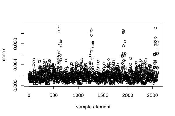
Figure 5.4: Cook’s distance for each sample observation
##         1         2         3         4         5         6         7         8
## 0.0008667 0.0013961 0.0013979 0.0010179 0.0016359 0.0016423 0.0018452 0.0013093
##         9        10
## 0.0021197 0.0012425
Another statistic that measures the degree of influence of an observation is DFBETA, denoted as \(D_f\text{Beta}_{(k)j}\), which measures the change in the regression coefficient \(\hat{\beta}_{j}\) when observation \(k\) is removed from the estimation process. Consequently, this measure evaluates the individual influence of each observation on the model parameters, identifying units whose presence substantially alters the estimates obtained. High values of \(D_f\text{Beta}_{(k)j}\) indicate that the observation exerts considerable influence on the corresponding coefficient, which can affect the stability and interpretation of the model.
According to Li & Valliant (2015), as a practical diagnostic criterion, an observation is usually considered influential for the coefficient \(\hat{\beta}_{j}\) when
\[ \left|D_f\text{Beta}_{(k)j}\right| \geq \frac{z}{\sqrt{n_I\times DEFF}}, \]
where \(z\) commonly takes values of 2 or 3, \(n_I\) represents the number of PSUs selected in the first-stage sample, and \(DEFF\) corresponds to the design effect. The influence of the observations on the coefficients of the example model is evaluated below using the svydfbetas function. The results corresponding to the first ten observations are presented in Table 5.1.
d_dfbetas <- data.frame(t(svydfbetas(fit_svy)$Dfbetas))
colnames(d_dfbetas) <- paste0("Beta_", 1:4)
d_dfbetas %>%
slice(1:10L)| Beta_1 | Beta_2 | Beta_3 | Beta_4 |
|---|---|---|---|
| 0.000 | 0 | 0.001 | -0.003 |
| -0.001 | 0 | 0.001 | 0.002 |
| -0.001 | 0 | 0.001 | 0.002 |
| 0.000 | 0 | 0.001 | -0.003 |
| -0.001 | 0 | 0.001 | 0.002 |
| 0.003 | 0 | -0.003 | -0.008 |
| 0.003 | 0 | -0.003 | -0.008 |
| 0.000 | 0 | -0.003 | 0.008 |
| 0.003 | 0 | -0.003 | -0.008 |
| -0.001 | 0 | 0.001 | -0.003 |
Once the values of the DFBETA measure have been obtained for each observation and model coefficient, the corresponding influence threshold is calculated from the results generated by the svydfbetas function. Based on this criterion, a dichotomous variable is constructed to classify observations according to their level of influence on the model estimates. The results of this classification are presented in Table 5.2.
d_dfbetas$id <- 1:nrow(d_dfbetas)
d_dfbetas <- reshape2::melt(d_dfbetas, id.vars = "id")
cutoff <- svydfbetas(fit_svy)$cutoff
d_dfbetas <- d_dfbetas %>%
  mutate(criterion = ifelse(abs(value) > cutoff, "Yes", "No"))

label_text <- d_dfbetas %>%
  filter(criterion == "Yes") %>%
  arrange(desc(abs(value))) %>%
  slice(1:10L)

label_text| id | variable | value | criterion |
|---|---|---|---|
| 889 | Beta_1 | 0.284 | Yes |
| 891 | Beta_1 | 0.284 | Yes |
| 890 | Beta_2 | -0.280 | Yes |
| 889 | Beta_2 | -0.275 | Yes |
| 891 | Beta_2 | -0.275 | Yes |
| 890 | Beta_1 | 0.250 | Yes |
| 890 | Beta_3 | 0.161 | Yes |
| 890 | Beta_4 | 0.158 | Yes |
| 889 | Beta_3 | 0.156 | Yes |
| 891 | Beta_3 | 0.156 | Yes |
The results show that several observations exceed the threshold established by the \(D_f\text{Beta}_{(k)j}\) criterion, indicating that these units exert substantial influence on the estimation of some model coefficients and suggesting the presence of units with high impact on the stability of the fit. Figure 5.5 presents the graphical representation of the \(D_f\)Beta values together with the reference threshold used to identify influential observations. In the figure, the points highlighted in red correspond to the observations that exceed this threshold and therefore require more detailed review within the model diagnostic process.
ggplot(d_dfbetas, aes(y = abs(value), x = id)) +
  geom_point(aes(col = criterion)) +
  geom_text(
    data = label_text,
    angle = 45,
    vjust = -1,
    aes(label = id)
  ) +
  geom_hline(aes(yintercept = cutoff)) +
  facet_wrap(. ~ variable, nrow = 2) +
  scale_color_manual(
    values = c("Yes" = "red", "No" = "black")
  )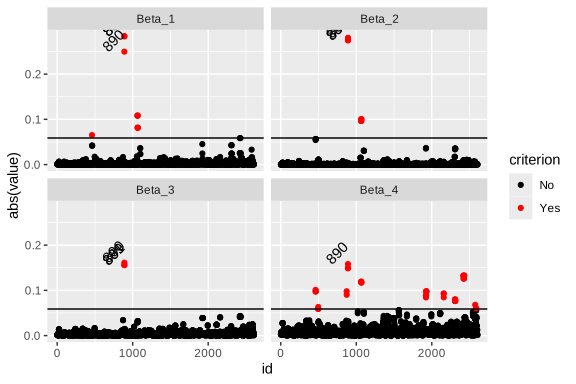
Figure 5.5: DfBetas values by parameter: influential observations indicated in red
Finally, the DFFITS statistic, denoted by \(D_f\text{Fits}_{(k)}\), measures the influence that observation \(k\) exerts on the fitted values of the model. In particular, this statistic evaluates how much the model predictions change when an observation is removed from the estimation process. Consequently, high values of \(D_f\text{Fits}_{(k)}\) indicate observations capable of substantially altering the overall model fit and, therefore, potentially influential in the inference process. According to Li & Valliant (2015), an observation is considered influential if:
\[ |D_f\text{Fits}_{(k)}| \geq z\sqrt{\frac{p}{n\times DEFF}} \] where \(z\) commonly takes values of 2 or 3, while \(n\) represents the total sample size of elements included in the survey. In the context of complex surveys, the use of thresholds adjusted by the design effect is especially relevant, since it incorporates the loss of precision derived from stratification, clustering, and the use of unequal weights.
In R, this statistic can be calculated using the svydffits function from the svydiags package, which obtains influence measures while explicitly considering the structure of the sampling design. The corresponding graphical results are presented in Figure 5.6, where the existence of some influential observations is confirmed (indicated in red).
d_dffits <- data.frame(
  dffits = svydffits(fit_svy)$Dffits,
  id = 1:length(svydffits(fit_svy)$Dffits)
)
cutoff <- svydffits(fit_svy)$cutoff
d_dffits <- d_dffits %>%
  mutate(cutoff_criterion = ifelse(abs(dffits) > cutoff, "Yes", "No"))

ggplot(d_dffits, aes(y = abs(dffits), x = id)) +
  geom_point(aes(col = cutoff_criterion)) +
  geom_hline(yintercept = cutoff) +
  scale_color_manual(
    values = c("Yes" = "red", "No" = "black")
  )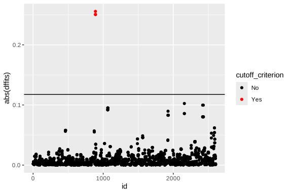
Figure 5.6: DfFits values: influential observations on the overall fit indicated in red
5.5 Inference about model parameters
Once the model fit has been evaluated and the fulfillment of the assumptions associated with the errors has been checked, the next step is to determine the statistical significance of the estimated parameters. This analysis makes it possible to establish whether the covariates included in the model provide relevant information for explaining the variability of the response variable.
In models fitted with data from complex surveys, hypothesis tests for regression coefficients are constructed using variance estimators that are consistent with the sampling design. To evaluate the effect of a covariate associated with the parameter \(\beta_j\), the following contrast is usually considered
\[ H_0:\beta_j=0 \qquad \text{frente a} \qquad H_1:\beta_j\neq 0. \]
The corresponding test statistic is defined as
\[ t_j= \frac{\hat{\beta}_{j}-\beta_{j}} {\sqrt{\widehat{Var}(\hat{\beta}_{j})}} \]
which, under the null hypothesis, approximately follows a Student’s \(t\) distribution with \(df\) degrees of freedom associated with the sampling design (usually defined as the number of primary sampling units minus the number of strata). The inferential decision is based on comparing the absolute value of the statistic \(t_j\) with the critical value of the reference distribution. When the observed value of the statistic is sufficiently large in magnitude, the null hypothesis is rejected and it is concluded that the corresponding covariate has a statistically significant association with the response variable.
The same distributional properties make it possible to construct confidence intervals for the regression coefficients. Thus, a confidence interval at the \((1-\alpha)\times100\%\) level for the parameter \(\beta_j\) is given by
\[ \hat{\beta}_{j} \pm t_{1-\frac{\alpha}{2},\,df} \sqrt{\widehat{Var}(\hat{\beta}_{j})}, \]
where \(t_{1-\frac{\alpha}{2},\,df}\) represents the quantile of order \(1-\alpha/2\) of the Student’s \(t\) distribution with \(df\) degrees of freedom.
To implement these procedures in R, the functions summary.svyglm and confint.svyglm are used; these make it possible to obtain, respectively, significance tests based on the \(t\) statistic and confidence intervals for the coefficients estimated under the complex sampling design. The corresponding results are presented in Table 5.3.
summary_table <- summary(fit_svy)$coefficients %>%
  as.data.frame() %>%
tibble::rownames_to_column("Parameter")| Parameter | Estimate | Std. Error | t value | Pr(>|t|) |
|---|---|---|---|---|
| (Intercept) | 73.580 | 59.470 | 1.237 | 0.218 |
| Expenditure | 1.222 | 0.197 | 6.212 | 0.000 |
| ZoneUrban | 66.652 | 39.666 | 1.680 | 0.096 |
| SexMale | 20.644 | 15.611 | 1.322 | 0.189 |
The model results indicate that the variable Expenditure has a statistically significant association with the variable of interest (Income). This effect is highly statistically significant (\(p < 0.001\)), providing strong evidence of a positive linear relationship between the two variables. In turn, for the categorical variables ZoneUrban and SexMale, the level of statistical significance is marginal (\(p = 0.096\) and \(p = 0.189\), respectively), so the evidence is not conclusive at the conventional 5% level.
5.6 Estimation and prediction
According to Heeringa et al. (2017), regression models serve two fundamental objectives. The first is to explain the variability of the response variable using the available covariates, a purpose that has been developed throughout this chapter. The second corresponds to predicting the expected value of the variable of interest for new observations, both within and outside the sample domain. The following expression represents the expected value of the response variable \(y_k\) conditional on the observed covariate vector \(\mathbf{x}_{k}\). In other words, the model uses the available information from the explanatory variables to estimate the expected average value of the variable of interest for unit \(i\).
\[ \hat \mu_k = \hat{E}(y_{k}\mid\mathbf{x}_{k})=\mathbf{x}_{k}\hat{\boldsymbol{\beta}} \]
Likewise, the variance associated with the estimation of the expected value, defined as \({Var}(\hat{\mu}_k) = {Var}(\mathbf{x}_{k}\hat{\boldsymbol{\beta}})\), can be estimated using the following expression:
\[ \widehat{Var}(\hat \mu_k) = \mathbf{x}'_{k}\ \hat{\boldsymbol{\Sigma}}\ \mathbf{x}_{k} \]
Here, \(\hat{\boldsymbol{\Sigma}}=\widehat{Var}(\hat{\boldsymbol{\beta}})\) corresponds to the estimated variance-covariance matrix of the regression model parameters. This expression quantifies the uncertainty associated with the prediction obtained for unit \(k\), simultaneously considering the variability of each estimated coefficient and the correlation between them. Consequently, units whose covariate values are associated with regions of greater uncertainty in coefficient estimation will have higher variances. Therefore, the precision of the estimates depends directly on the precision with which the regression model coefficients are estimated. Continuing with the example model, recall that the estimated model coefficients are presented in Table 5.4:
The model coefficients are converted to a tidy table using broom::tidy() (Robinson et al., 2026), which makes it easier to present estimates, standard errors, and tests in a rectangular structure.
| term | estimate | std.error | statistic | p.value |
|---|---|---|---|---|
| (Intercept) | 73.580 | 59.470 | 1.237 | 0.218 |
| Expenditure | 1.222 | 0.197 | 6.212 | 0.000 |
| ZoneUrban | 66.652 | 39.666 | 1.680 | 0.096 |
| SexMale | 20.644 | 15.611 | 1.322 | 0.189 |
Based on the estimated model coefficients, the estimate of the expected value of the response variable for unit \(k\) can be expressed as:
\[ \hat{E}(y_{k}\mid\mathbf{x}_{k})=73.58+1.22 \times x_{1i}+66.65 \times x_{2i}+20.64 \times x_{3i} \]
The following code calculates the regression model predictions for the observations included in the sample, using the design matrix and the vector of estimated coefficients:
x_obs <- model.matrix(fit_svy) %>%
  data.frame() %>%
  as.matrix()
hat_beta <- fit_svy$coe
hat_mu <- as.numeric(x_obs %*% hat_beta)
hat_mu %>%
  head(10)
## [1] 517.6 496.9 496.9 517.6 496.9 553.1 553.1 573.7 553.1 184.8First, the instruction model.matrix(fit_svy) constructs the design matrix associated with the fitted model, automatically incorporating the explanatory variables. Next, the object hat_beta stores the vector of estimated regression model coefficients. The estimates are then obtained through the matrix product x_obs %*% hat_beta. Finally, the function head(10) makes it possible to view the first ten estimates obtained.
To calculate the variance of the estimates, the variance-covariance matrix of the model parameters is required. The elements of the main diagonal correspond to the variances of the estimated parameters, while the off-diagonal elements represent the covariances between pairs of coefficients. The estimated variance-covariance matrix is presented in Table 5.5:
| Parameter | (Intercept) | Expenditure | ZoneUrban | SexMale |
|---|---|---|---|---|
| (Intercept) | 3536.68 | -10.551 | 123.689 | 326.13 |
| Expenditure | -10.55 | 0.039 | -3.295 | -0.57 |
| ZoneUrban | 123.69 | -3.295 | 1573.353 | -121.45 |
| SexMale | 326.13 | -0.570 | -121.446 | 243.72 |
In computational terms, this involves combining the covariate vector for each observation with the matrix \(\hat{\boldsymbol{\Sigma}}\) to obtain the precision of the individual predictions. The following code calculates the variance associated with the predictions obtained from the regression model:
cov_beta <- vcov(fit_svy) %>%
  as.matrix()
mu_variance <- as.numeric(x_obs %*% cov_beta %*% t(x_obs))
mu_variance %>%
  head(10)
## [1] 1374.9 1002.6 1002.6 1374.9 1002.6 1107.8 1107.8 1480.1 1107.8 750.8The confidence interval, which provides a range of plausible values for the expected value of the response variable conditional on the observed covariates, is obtained by:
\[ \mathbf{x}_{k}\hat{\beta}\pm t_{\left(1-\frac{\alpha}{2},df\right)}\sqrt{\mathbf{x}'_{k} \ \hat{\boldsymbol{\Sigma}} \ \mathbf{x}_{k}} \]
In R, the function predict(fit_svy, type = "link") generates the linear predictions of the fitted model. The argument type = "link" indicates that the estimates are obtained on the scale of the linear predictor, that is, using directly the linear combination of the covariates and the estimated coefficients. The function confint() then calculates the confidence intervals associated with these predictions.
hat_mu <- data.frame(predict(fit_svy, type = "link"))
mu_ci <- data.frame(confint(predict(fit_svy, type = "link")))
colnames(mu_ci) <- c("lower_limit", "upper_limit")
The estimates obtained from the model, together with their respective confidence intervals, can be visualized graphically in Figure 5.7.
pred <- cbind(hat_mu, mu_ci)
pred$Expenditure <- survey_data$Expenditure
pd <- position_dodge(width = 0.2)
ggplot(
  pred %>%
    slice(1:100L),
  aes(x = Expenditure, y = link)
) +
  geom_errorbar(
    aes(ymin = lower_limit, ymax = upper_limit),
    width = .1,
    linetype = 1
  ) +
  geom_point(size = 2, position = pd) +
  theme_bw()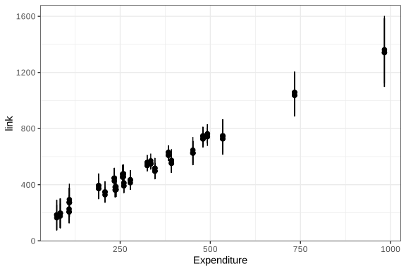
Figure 5.7: Point predictions and confidence intervals for the first 100 sample observations
When the interest is in making predictions for covariate values that fall outside the range observed in the sample, the uncertainty associated with the estimate increases. In these cases, it is not enough to consider only the variability derived from estimating the model parameters; the variability inherent to the random term of the regression must also be incorporated. For this reason, the prediction variance includes an additional component associated with the residual error of the model:
\[ \widehat{Var}\left[\hat{E}\left(y_{k}\mid\mathbf{x}_{k}\right)\right] = \mathbf{x}'_{k} \ \hat{\boldsymbol{\Sigma}} \ \mathbf{x}_{k} + \hat{\sigma}^2_{yx} \]
In this expression, the term \(\hat{\sigma}^2_{yx}\) corresponds to the estimated residual variance, that is, the part of the variability of the response variable that is not explained by the covariates included in the model. Incorporating this second component is fundamental when predicting for unobserved units, since it explicitly recognizes the existence of individual variability around the estimated mean.
Consequently, prediction intervals are usually wider than confidence intervals for the mean, reflecting greater uncertainty associated with the prediction of individual values. Thus, the prediction interval for a new observation can be expressed as:
\[ \mathbf{x}_{k}\hat{\boldsymbol{\beta}} \pm t_{\left(1-\frac{\alpha}{2},df\right)} \sqrt{ \mathbf{x}_{k}^{t} \hat{\boldsymbol{\Sigma}}_{\hat{\boldsymbol{\beta}}} \mathbf{x}_{k} + \hat{\sigma}^2_{yx} } \]
Suppose, for example, that the goal is to obtain the model prediction for a new observation corresponding to a male individual (Male), residing in an urban area (Urban), with an expenditure level (Expenditure) equal to 1600. This profile can be defined in R using the following data set:
new_data <- data.frame(
  Expenditure = 1600,
  Sex = "Male",
  Zone = "Urban"
)

predict(fit_svy, newdata = new_data, type = "link")
## link SE
## 1 2117 243## 2.5 % 97.5 %
## 1 1641 2593First, the object new_data specifies the values of the covariates included in the model. The function predict() then calculates the point prediction associated with that observation. The argument newdata = new_data indicates that the prediction should be made using the new information supplied, while type = "link" requests the result on the scale of the linear predictor. Finally, the function confint() makes it possible to obtain the confidence interval associated with the prediction made. This interval quantifies the uncertainty of the estimate and provides a range of plausible values for the expected value of the response variable corresponding to the specified profile.