Chapter 7 Multilevel Models
Multilevel models, also known as hierarchical models, are a statistical technique designed for the analysis of data with a hierarchical structure, such as those from household surveys, where the observation units are not independent of each other. Individuals belong to households, households are located in specific geographic areas (PSUs) and these, in turn, are part of broader territorial units (strata or domains). As a consequence, observations that share the same context tend to present characteristics that are more similar to each other than those belonging to different contexts. This dependence structure violates one of the fundamental assumptions of conventional regression models and can lead to inefficient estimates and incorrect inferences.
Unlike conventional regression models, multilevel models recognize that observations can be grouped at different levels and that each of them can contribute to explaining the observed variability. Consequently, they allow the effects associated with the characteristics of the units of analysis and those derived from the environment or context in which they are located to be simultaneously represented. This formulation is especially useful when seeking to study phenomena determined both by individual factors and by characteristics of households, communities, or geographic areas.
Another important feature of multilevel models is that they make it possible to quantify the proportion of variability associated with each level of grouping present in the data. While fixed effects summarize the average relationship between the response variable and the covariates included in the model, random effects represent systematic differences between groups that are not explained by these covariates. Thanks to this structure, it is possible to explicitly model the dependence between observations belonging to the same group and obtain more appropriate inferences when the data have a hierarchical organization.
The theoretical and methodological development of multilevel models has been widely documented in the sampling literature. Among the most influential references are the works of Goldstein (2011), Gelman & Hill (2006), and Rabe-Hesketh & Skrondal (2012), which present the conceptual foundations, estimation strategies, and various applications of these models in social and demographic contexts. In addition, Browne & Draper (2006) compare different estimation approaches for hierarchical models, evaluating the differences between methods based on maximum likelihood and Bayesian approaches. In the field of social epidemiology, Merlo et al. (2006) emphasize the usefulness of multilevel models for studying contextual phenomena, showing how factors associated with the environment can contribute to explaining inequalities in health and other outcomes of population interest.
7.1 Motivation
To begin this chapter, tidyverse (Wickham, Averick, et al., 2026) is loaded for data manipulation and graph production, and lme4 (Bates et al., 2026) for multilevel model estimation. The database that will be used throughout the examples is imported. The mathematical titles of some figures are formatted with latex2exp (Meschiari, 2026), called explicitly in the code.
survey_data <- readRDS("Data/encuesta.rds") %>%
  mutate(poverty = ifelse(Poverty != "NotPoor", 1, 0))
For illustrative purposes, the examples in this section are developed from a subsample of the survey. The following code block builds the database used in the chapter examples. To do so, it identifies the three strata with the smallest number of households and retains only the variables required for the analysis: income, expenditure, stratum, sex, region, area of residence, and poverty status.
plot_data <- survey_data %>%
  select(HHID, Stratum) %>%
  distinct() %>%
  group_by(Stratum) %>%
  tally() %>%
  arrange(n) %>%
  select(-n) %>%
  slice(1:3L) %>%
  inner_join(survey_data, by = "Stratum") %>%
  select(Income, Expenditure, Stratum, Sex, Region, Zone, poverty)
As a starting point, a conventional linear regression model is fitted that relates household income to household expenditure, temporarily ignoring the hierarchical structure of the data. Under this specification, it is assumed that all observations are independent and that the relationship between income and expenditure is homogeneous for all households, regardless of the stratum to which they belong. Figure 7.1 presents the estimated regression line along with the observed data.
ggplot(data = plot_data,
       aes(y = Income, x = Expenditure)) +
  geom_jitter() +
  geom_smooth(formula = y ~ x, method = "lm", se = FALSE) +
  ggtitle(latex2exp::TeX(
    "$Income_{i} \\sim \\hat{\\beta}_{0} + \\hat{\\beta}_{1}Expenditure_{i} + \\epsilon_{i}$"
  )) +
  theme(
    legend.position = "none",
    plot.title = element_text(hjust = 0.5)
  )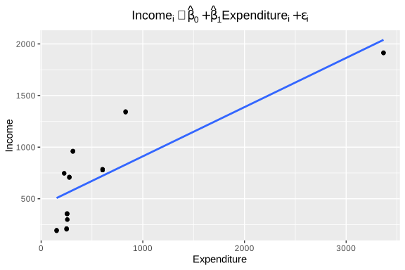
Figure 7.1: Simple linear regression model for income as a function of expenditure (without considering strata)
While this model is useful as an initial reference, its assumptions are often unrealistic in the context of household surveys. In particular, independence between observations may be compromised when households belong to strata that share similar socioeconomic, demographic, or geographic characteristics. Likewise, it is possible that average income levels differ systematically between strata, even when the relationship between income and expenditure is similar. As Finch et al. (2019) point out, ignoring this hierarchical structure can lead to incorrect estimates of standard errors and, consequently, unreliable statistical inferences.
For illustrative purposes only, the hierarchical structure of the data is gradually incorporated into the modeling process. To do so, a model is initially fitted that allows each stratum to have its own intercept, while maintaining a common slope for all observations. This specification is useful for visualizing how average income levels may differ between strata, even when the relationship between income and expenditure is considered constant.
beta_1 <- coef(lm(Income ~ Expenditure, data = plot_data))[2]
model_coef <- plot_data %>%
  group_by(Stratum) %>%
  summarise(beta_0 = coef(lm(Income ~ Expenditure))[1]) %>%
  mutate(beta_1 = beta_1)
In this way, the model introduces a first source of heterogeneity between groups and makes it possible to appreciate the limitations of the simple regression model presented previously, which assumed a single regression line for the entire population. Figure 7.2 presents the regression lines with intercepts differentiated by stratum:
ggplot(data = plot_data,
       aes(y = Income, x = Expenditure, colour = Stratum)) +
  geom_jitter() +
  geom_abline(data = model_coef,
              mapping = aes(slope = beta_1, intercept = beta_0, colour = Stratum)) +
  ggtitle(latex2exp::TeX(
    "$Income_{kj} \\sim \\hat{\\beta}_{0j} + \\hat{\\beta}_{1}Expenditure_{kj} + \\epsilon_{kj}$"
  )) +
  theme(
    legend.position = "none",
    plot.title = element_text(hjust = 0.5)
  )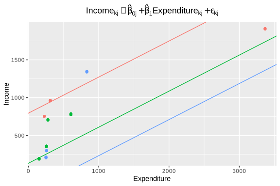
Figure 7.2: Model with stratum-specific intercept and common slope
As a next step, an alternative specification is considered in which all strata share the same average level of income, represented by a common intercept, but the relationship between income and expenditure is allowed to vary between strata through slopes specific to each stratum.
beta_0 <- coef(lm(Income ~ Expenditure, data = plot_data))[1]
model_coef <- plot_data %>%
  group_by(Stratum) %>%
  summarise(beta_1 = coef(lm(Income ~ Expenditure))[2]) %>%
  mutate(beta_0 = beta_0)
Under this specification, the differences between strata are manifested in the intensity of the association between income and expenditure, rather than in their average levels. Figure 7.3 makes it possible to visualize these differences in the estimated regression trajectories for each stratum.
ggplot(data = plot_data,
       aes(y = Income, x = Expenditure, colour = Stratum)) +
  geom_jitter() +
  geom_abline(data = model_coef,
              mapping = aes(slope = beta_1, intercept = beta_0, colour = Stratum)) +
  ggtitle(latex2exp::TeX(
    "$Income_{kj} \\sim \\hat{\\beta}_{0} + \\hat{\\beta}_{1j}Expenditure_{kj} + \\epsilon_{kj}$"
  )) +
  theme(
    legend.position = "none",
    plot.title = element_text(hjust = 0.5)
  )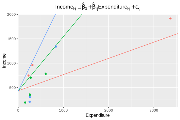
Figure 7.3: Model with stratum-specific slope and common intercept
Finally, the most flexible specification of those presented so far is considered, allowing both the average level of income and the relationship between income and expenditure to vary between strata. Under this approach, each stratum has its own regression line, with intercepts and slopes estimated independently.
model_coef <- plot_data %>%
  group_by(Stratum) %>%
  summarise(
    beta_0 = coef(lm(Income ~ Expenditure))[1],
    beta_1 = coef(lm(Income ~ Expenditure))[2]
  )
This formulation makes it possible to capture simultaneously differences in income levels and in the strength of their association with expenditure. Figure 7.4 shows the fitted lines for each stratum under this specification.
ggplot(data = plot_data,
       aes(y = Income, x = Expenditure, colour = Stratum)) +
  geom_jitter() +
  geom_abline(data = model_coef,
              mapping = aes(slope = beta_1, intercept = beta_0, colour = Stratum)) +
  ggtitle(latex2exp::TeX(
    "$Income_{kj} \\sim \\hat{\\beta}_{0j} + \\hat{\\beta}_{1j}Expenditure_{kj} + \\epsilon_{kj}$"
  )) +
  theme(
    legend.position = "none",
    plot.title = element_text(hjust = 0.5)
  )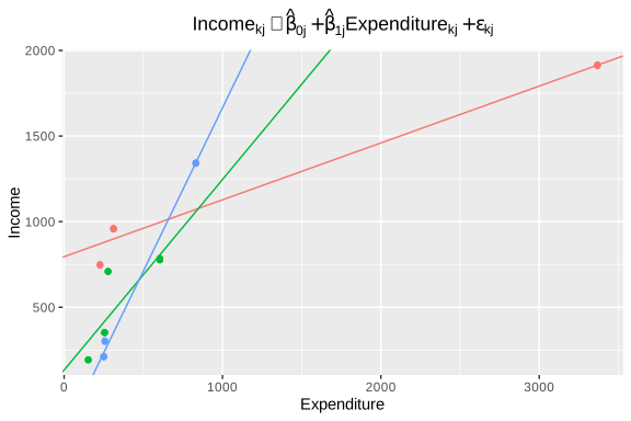
Figure 7.4: Model with stratum-specific intercept and slope (independent fit)
Although this last specification offers a more flexible representation of the data and allows the particular features of each stratum to be captured, it presents an important limitation: the parameters are estimated completely independently for each group. As a consequence, it does not take advantage of information shared across strata that may exhibit similar patterns, which can generate unstable estimates, especially in those groups with a small number of observations.
Multilevel models overcome this difficulty through a mechanism known as shrinkage, in which specific estimates for each group are obtained by combining the group’s own information with information from the population as a whole. In this way, a balance is achieved between the representation of the differences between strata and the statistical efficiency of the estimates.
7.2 q-weighted Weights
Regarding the incorporation of sampling weights in multilevel models, although there is a general consensus on the need to use them to guarantee inferences that are representative of the target population (Cai, 2013), there is no single methodological strategy for their implementation. In this context, Pfeffermann et al. (1998) and Asparouhov (2006) propose approaches based on pseudo-maximum likelihood, particularly through weighted generalized least squares procedures. Alternatively, Rabe-Hesketh & Skrondal (2006) propose methods based on EM algorithms for the estimation of hierarchical models with weights.
From a general perspective, the maximum likelihood approach consists of estimating the parameters of the model by identifying those values that maximize the probability of observing the available data under the assumed specification. An important extension of this approach is restricted maximum likelihood (REML), which improves the estimation of variance components by correcting the bias associated with the estimation of degrees of freedom, producing in many cases more stable estimates than conventional maximum likelihood (Kreft & De Leeuw, 1998).
In the context of multilevel models with survey data, an additional difficulty lies in the coherent incorporation of sampling weights across the different levels of the hierarchy. As Pfeffermann et al. (1998) point out, the clustered structure of the data implies that the observations are not independent, so the log-likelihood function cannot be decomposed as a simple sum of individual contributions. Instead, it is necessary to explicitly consider the dependence between the different levels of the sample design in order to obtain appropriate inferences.
To fit a multilevel model with data from complex surveys, it is recommended to redefine the expansion factors using the q-weighted weights approach proposed by Pfeffermann (2011). This procedure seeks to eliminate the systematic part of the weights associated with the covariates included in the model, preserving only the residual component of the selection mechanisms. The steps are as follows:
Fit a regression model for the final expansion factors of the survey, using as explanatory variables the same set of covariates that will be used in the multilevel model. Let \(w_k\) be the original expansion factor of unit \(k\) and \(\mathbf{x}_k\) the vector of covariates. Then the following model is fitted
\[ w_k = f(\mathbf{x}_k, \boldsymbol{\beta}) + \varepsilon_k, \]
where \(f(\cdot)\) represents the functional relationship between the weights \(w_k\) and the covariates \(\mathbf{x}_k\), through the coefficients \(\boldsymbol{\beta}\).
Obtain the predicted values from the model for each observation unit, such that:
\[ \hat{w}_k = f(\mathbf{x}_k, \hat{\boldsymbol{\beta}}). \]
These values represent the component of the expansion factors explained by the covariates included in the model.
Construct the q-weighted weights by dividing the original expansion factors by their corresponding predicted values,
\[ q_k = \frac{w_k}{\hat{w}_k}. \]
In this way, the new weights reflect only the residual variation of the expansion factors after controlling for the effect of the covariates.
Define the new sample design using the adjusted weights \(q_k\) instead of the original weights \(w_k\), and use this design to estimate the parameters of the multilevel model.
The following code implements the q-weighted weight construction procedure. First, it fits a linear regression model that explains the original expansion factors based on the explanatory variable expenditure. In this way, the resulting weights retain only the component of variation not explained by the covariates included in the multilevel model.
7.3 Linear Multilevel Model
The multilevel models most commonly used in practice are extensions of the classical linear model for data with a hierarchical structure. In their basic formulation, these models assume that the response variable is continuous and follows a normal distribution conditional on the fixed and random effects included in the model. It is also assumed that the random effects and residual errors are independent of each other and normally distributed with zero mean and constant variances.
7.3.1 Null Model
In multilevel regression analysis, two types of parameters are distinguished: regression coefficients, known as fixed parameters, and variance components associated with random effects. A fundamental initial stage in this type of analysis consists of decomposing the total variability of the dependent variable into the different levels of the hierarchical structure. In the context of the previous example, this decomposition makes it possible to separate income variation into a component attributable to differences within strata and another associated with differences between strata.
The starting point for this decomposition is the so-called null model, which does not incorporate explanatory variables and is expressed as
\[ y_{kj} = \beta_{0j} + \epsilon_{kj} \]
where \(y_{kj}\) denotes the observed value of income for unit \(k\) in stratum \(j\). The term \(\beta_{0j}\) represents the stratum-specific intercept, capturing the differences in the average levels of the variable between groups. Finally, \(\epsilon_{kj}\) corresponds to the error at the unit level, which captures the unexplained variability within each stratum and is assumed to have zero mean and constant variance conditional on the group.
In turn, the stratum intercept can be decomposed into a part common to all strata and a specific deviation for each of them, as follows:
\[ \beta_{0j} = \gamma_{00} + \tau_{0j} \]
where \(\gamma_{00}\) represents the global average intercept and \(\tau_{0j}\) is the random effect for the intercept that captures the deviation of stratum \(j\), allowing the heterogeneity between strata to be explicitly modeled. Furthermore, the random components of the model are assumed normally distributed with zero mean and specific variances for each level of the hierarchy. In particular, the random effect associated with the intercept by stratum satisfies
\[ \tau_{0j} \sim N\left(0, \sigma_{\tau}^{2}\right), \]
which implies that the deviations of each stratum from the global intercept are distributed around zero, with a variability determined by \(\sigma_{\tau}^{2}\). Analogously, the unit-level error term follows the distribution
\[ \epsilon_{kj} \sim N\left(0, \sigma_{\epsilon}^{2}\right), \]
where \(\sigma_{\epsilon}^{2}\) represents the residual variability within the strata. From this model, the intraclass correlation coefficient (ICC) is defined, which quantifies the proportion of the total variance explained by the differences between strata:
\[ \rho = \frac{\sigma_{\tau}^{2}}{\sigma_{\tau}^{2} + \sigma_{\epsilon}^{2}} \]
A high ICC value indicates that a significant proportion of the total variability of the variable of interest is due to differences between strata, which suggests the presence of relevant heterogeneity between groups and the need to explicitly incorporate that structure in the model. In contrast, a low ICC implies that the variability is mainly concentrated within the strata, which show greater relative homogeneity among themselves.
Continuing with the analysis of the example survey, when the variable of interest is income, the null model is the starting point for quantifying what proportion of the total variability is due to differences between strata and what proportion corresponds to differences between households within the same stratum.
Estimation of multilevel models in R is performed using the lme4 (Bates et al., 2026) package. In particular, the lmer() function makes it possible to specify random effects using expressions of the form (effect | group). In this context, the expression (1 | Stratum) indicates that the model includes a random intercept for each stratum. The value 1 represents the model intercept, while Stratum identifies the grouping variable.
Table 7.1 presents the estimated intercepts for each stratum from the null model. Since this model does not incorporate explanatory variables, each intercept can be interpreted as the expected average income in the corresponding stratum. The results show substantial differences between groups: while the idStrt004 stratum presents the highest estimated average income (959.6), the idStrt009 stratum registers the lowest value (207.6). These differences suggest the existence of substantial variability between strata, justifying the incorporation of random effects to explicitly model the hierarchical structure of the data.
| (Intercept) | |
|---|---|
| idStrt001 | 635 |
| idStrt002 | 507 |
| idStrt003 | 486 |
| idStrt004 | 960 |
| idStrt005 | 518 |
| idStrt006 | 439 |
| idStrt007 | 477 |
| idStrt008 | 377 |
| idStrt009 | 218 |
| idStrt010 | 594 |
| idStrt011 | 590 |
| idStrt012 | 362 |
Based on the variance components estimated in the null model, the intraclass correlation is calculated using the icc() function from the performance (Lüdecke et al., 2026) package. This indicator quantifies the proportion of total income variability that can be attributed to differences between strata, constituting a measure of the dependence between observations belonging to the same group. The results obtained are presented in Table 7.2.
| ICC_adjusted | ICC_unadjusted | optional |
|---|---|---|
| 0.329 | 0.329 | FALSE |
The estimated intraclass correlation of 32% indicates that approximately one third of the total observed variability in income is due to differences between strata, while the remaining percentage corresponds to differences between households within the same strata. Finally, since the null model does not include any predictors, the estimate of income within each stratum is constant and equal to the estimated intercept for that stratum.
7.3.2 Random Intercept Model
The simplest multilevel model that incorporates covariates is the random intercept model. In this specification, it is assumed that the effects of the explanatory variables are common to all strata, while the average level of the response variable may vary between them. The model is expressed as
\[ y_{kj} = \beta_{0j} + \mathbf{x}_{kj}\boldsymbol{\beta} + \epsilon_{kj} \]
where \(y_{kj}\) represents the observed value of the response variable for unit \(k\) belonging to stratum \(j\), \(\mathbf{x}_{kj}\) is the vector of covariates associated with that unit, \(\boldsymbol{\beta}\) is the vector of regression coefficients common to all strata and \(\epsilon_{kj}\) corresponds to the random error at the unit level.
As in the null model, the intercept is modeled as \(\beta_{0j} = \gamma_{00} + \tau_{0j}\); where \(\gamma_{00}\) represents the global average intercept and \(\tau_{0j}\) is the random effect associated with stratum \(j\), which measures the deviation of that stratum from the overall average.
The random components of the model are assumed to be independent and normally distributed, so that \(\tau_{0j} \sim N(0,\sigma_{\tau}^{2})\) and \(\epsilon_{kj} \sim N(0,\sigma_{\epsilon}^{2})\). Under these conditions, the total variability of the response variable can be decomposed into a component between strata, quantified by \(\sigma_{\tau}^{2}\), and a component within the strata, represented by \(\sigma_{\epsilon}^{2}\).
The following code fits a multilevel random intercept model, where income (Income) is explained by household expenditure (Expenditure), also incorporating a random effect associated with the stratum (Stratum) and using the q-weighted weights stored in the variable qk. Once the model is fitted, the intraclass correlation (ICC) is estimated from the estimated variance components.
random_intercept_model <- lmer(
  Income ~ Expenditure + (1 | Stratum),
  data = survey_data,
  weights = qk
)
performance::icc(random_intercept_model)
## # Intraclass Correlation Coefficient
##
## Adjusted ICC: 0.203
## Unadjusted ICC: 0.109The adjusted intraclass correlation of 0.196 indicates that, after controlling for household expenditure (Expenditure), approximately 20% of the residual variability in income remains attributable to differences between strata. Although this value is lower than that obtained with the null model, the magnitude of the ICC continues to justify the use of a multilevel model to adequately represent the hierarchical structure of the data. The estimated coefficients by stratum are presented in Table 7.3:
| (Intercept) | Expenditure | |
|---|---|---|
| idStrt001 | 250.4 | 1.19 |
| idStrt002 | 156.8 | 1.19 |
| idStrt003 | 142.9 | 1.19 |
| idStrt004 | 296.8 | 1.19 |
| idStrt005 | -32.4 | 1.19 |
| idStrt006 | 53.8 | 1.19 |
| idStrt007 | 12.5 | 1.19 |
| idStrt008 | 107.1 | 1.19 |
To facilitate the visualization of the model results, the reduced subsample presented above is used, which contains only three selected strata.
estimated_coef <- inner_join(
  coef(random_intercept_model)$Stratum %>%
    tibble::rownames_to_column(var = "Stratum"),
  plot_data %>%
    select(Stratum) %>%
    distinct()
)
Figure 7.5 shows the estimated regression lines for each stratum under the random intercept model. The lines share the same slope, reflecting the common effect of expenditure on income, but they differ in their vertical position due to the specific intercepts estimated for each stratum.
ggplot(data = plot_data,
       aes(y = Income, x = Expenditure, colour = Stratum)) +
  geom_jitter() +
  geom_abline(data = estimated_coef,
              mapping = aes(slope = Expenditure,
                            intercept = `(Intercept)`,
                            colour = Stratum)) +
  theme(
    legend.position = "none",
    plot.title = element_text(hjust = 0.5)
  )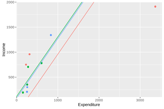
Figure 7.5: Estimated regression lines by stratum: model with random intercept
7.3.3 Random Intercept and Slope Model
A natural extension of the previous model is the random intercept and slope model. In this specification, not only is the average level of the response variable allowed to vary between strata, but the effect of one or more covariates is also allowed to differ between groups. In this way, each stratum can have its own regression line, both in terms of intercept and slope. The model can be expressed as
\[ y_{kj} = \beta_{0j} + x_{kj}\beta_{1j} + \mathbf{z}_{kj}\boldsymbol{\beta} + \epsilon_{kj}, \]
where \(y_{kj}\) represents the observed value of the response variable for unit \(k\) belonging to stratum \(j\), \(x_{kj}\) corresponds to the covariate whose slope is allowed to vary between strata, \(\mathbf{z}_{kj}\) contains the covariates with fixed effects common to all groups, and \(\epsilon_{kj}\) is the error term at the unit level. In this model, both the intercept and the slope associated with \(x_{kj}\) are considered random and are decomposed as follows:
\[ \beta_{0j} = \gamma_{00} + \tau_{0j}, \qquad \beta_{1j} = \gamma_{10} + \tau_{1j} \]
where \(\gamma_{00}\) and \(\gamma_{10}\) represent, respectively, the average intercept and slope in the population, while \(\tau_{0j}\) and \(\tau_{1j}\) capture the specific deviations of stratum \(j\) from those averages. These random effects are assumed normally distributed as follows:
\[ \begin{pmatrix} \tau_{0j} \\ \tau_{1j} \end{pmatrix} \sim N\left( \begin{pmatrix} 0 \\ 0 \end{pmatrix}, \begin{pmatrix} \sigma_{\tau_0}^2 & \sigma_{\tau_{01}} \\ \sigma_{\tau_{01}} & \sigma_{\tau_1}^2 \end{pmatrix} \right), \]
while the unit-level error satisfies \(\epsilon_{kj} \sim N(0,\sigma_{\epsilon}^{2})\). Consequently, the model makes it possible to quantify not only the variability between strata in the average levels of the response variable, but also the existing heterogeneity in the effect of the covariate whose coefficient is modeled as random.
The following code fits a multilevel model with random intercept and slope, in which income (Income) is explained by household expenditure (Expenditure) and area of residence (Zone). In this case, both the intercept and the effect of expenditure may vary between strata through random effects associated with Stratum, also using the q-weighted weights stored in the variable qk.
random_slope_model <- lmer(
  Income ~ 1 + Expenditure + (1 + Expenditure | Stratum),
  data = survey_data,
  weights = qk
)

performance::icc(random_slope_model)
## # Intraclass Correlation Coefficient
##
## Adjusted ICC: 0.690
## Unadjusted ICC: 0.457Note that the code specification simultaneously includes fixed effects and random effects for the intercept and the variable Expenditure. The terms outside the parentheses, 1 + Expenditure, correspond to the fixed effects of the model and make it possible to estimate the global average intercept and the global average slope associated with expenditure. For its part, the expression (1 + Expenditure | Stratum) incorporates the specific deviations of each stratum from those averages. The explicit inclusion of fixed effects is fundamental, since random effects are interpreted as deviations around a population mean. The model coefficients by stratum are presented in Table 7.4:
| (Intercept) | Expenditure | |
|---|---|---|
| idStrt001 | -222.8 | 2.730 |
| idStrt002 | 35.5 | 1.607 |
| idStrt003 | 151.9 | 1.164 |
| idStrt004 | 224.2 | 1.353 |
| idStrt005 | -89.7 | 1.286 |
| idStrt006 | 28.6 | 1.217 |
| idStrt007 | 41.0 | 1.079 |
| idStrt008 | 163.8 | 0.928 |
| idStrt009 | 16.6 | 0.838 |
| idStrt010 | 89.9 | 1.830 |
Once again, in order to facilitate the visualization of the results, the reduced subsample defined previously is used, which includes only three selected strata.
estimated_coef <- inner_join(
  coef(random_slope_model)$Stratum %>%
    tibble::rownames_to_column(var = "Stratum"),
  plot_data %>%
    select(Stratum) %>%
    distinct()
)
Figure 7.6 presents the estimated regression lines for each stratum under the random intercept and slope model. Unlike the random intercept model, in this case the lines differ both in their vertical position and in their slope, reflecting that strata not only have different average income levels, but also different strengths in the relationship between income and expenditure.
ggplot(data = plot_data,
       aes(y = Income, x = Expenditure, colour = Stratum)) +
  geom_jitter() +
  geom_abline(data = estimated_coef,
              mapping = aes(slope = Expenditure,
                            intercept = `(Intercept)`,
                            colour = Stratum)) +
  theme(
    legend.position = "none",
    plot.title = element_text(hjust = 0.5)
  )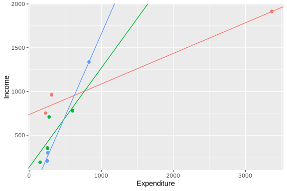
Figure 7.6: Estimated regression lines by stratum: model with random intercept and slope
7.4 Multilevel Logistic Model
Multilevel logistic models extend multilevel models for continuous variables to the case in which the response variable is dichotomous. Instead of directly modeling the expected value of a continuous variable, these models estimate the probability of occurrence of an event, simultaneously incorporating individual covariates and random effects associated with the groups to which units belong. In the context of household surveys, this formulation is especially useful when analyzing binary outcomes, such as being in poverty or not, accessing a service or not, participating or not in the labor market, or presenting a certain sociodemographic characteristic.
As in multilevel models for continuous variables, the starting point is to recognize that the observation units are not independent when they belong to the same stratum, cluster, or domain. However, in the logistic case the response is not represented by a normal distribution with an additive residual error, but by a Bernoulli distribution conditional on the probability of occurrence of the event. This probability is linked to the predictors through the logit function, which makes it possible to express the model on a linear scale.
\[ y_{kj} \mid \pi_{kj} \sim \text{Bernoulli}(\pi_{kj}) \]
where \(y_{kj}\) takes the value one if unit \(k\) of stratum \(j\) presents the event of interest and zero otherwise. The conditional probability of the event is denoted by \(\pi_{kj}=Pr(y_{kj}=1)\) and is related to the linear predictor through
\[ \text{logit}(\pi_{kj}) = \log\left(\frac{\pi_{kj}}{1-\pi_{kj}}\right) = \eta_{kj} \]
In this formulation, \(\eta_{kj}\) plays a role analogous to the linear expected value of models for continuous variables. The central difference is that the fixed and random effects act on the logit scale and not directly on the probability. Therefore, the differences between strata are interpreted as shifts in the log-odds of the event, which are then transformed into probabilities through the logistic function. Figure 7.7 presents the relationship between expenditure and the probability of poverty, with a fitted logistic curve.
ggplot(data = survey_data,
       aes(y = poverty, x = Expenditure)) +
  geom_point(alpha = 0.5) +
  geom_smooth(
    formula = y ~ x,
    method = "glm",
    se = FALSE,
    method.args = list(family = binomial(link = "logit"))
  ) +
  labs(y = "Poverty (1 = poor)", x = "Expenditure")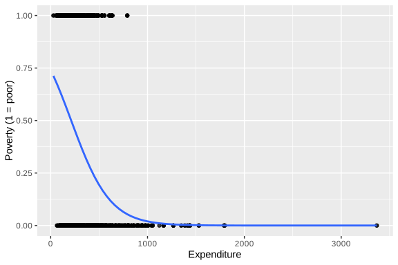
Figure 7.7: Relationship between expenditure and poverty status with fitted logistic curve
The fitted curve summarizes the marginal association between expenditure and poverty status, without yet incorporating the hierarchical structure of the strata. In general terms, the descending shape of the curve indicates that, as household expenditure increases, the estimated probability of being in poverty decreases. However, this average relationship can hide relevant differences between strata, especially when households belong to different socioeconomic contexts.
7.4.1 Logistic Null Model
As in the case of continuous variables, the logistic null model constitutes the starting point to study the hierarchical structure of the response variable. This model does not incorporate covariates and allows us to evaluate whether the average probability of the event varies between strata. In the example considered, the event of interest corresponds to the poverty status, so that the model allows us to separate the heterogeneity attributable to differences between strata from the individual variation inherent to a binary response.
In the null model, the variable of interest follows the following Bernoulli distribution:
\[ y_{kj} \mid \pi_{kj} \sim \text{Bernoulli}(\pi_{kj}) \]
where the probability of success for unit \(k\) belonging to group \(j\) is modeled through
\[ \text{logit}(\pi_{kj}) = \beta_{0j}, \]
where \(\beta_{0j}\) represents the specific intercept of stratum \(j\) on a logit scale. In turn, this intercept is decomposed as
\[ \beta_{0j} = \gamma_{00} + \tau_{0j} \]
where \(\gamma_{00}\) is the global average intercept of the population and \(\tau_{0j}\) the random effect associated with stratum \(j\), which captures the deviations of each group from the overall average. As in the null model for continuous variables, this random effect allows heterogeneity between groups to be explicitly modeled:
\[ \tau_{0j} \sim N(0,\sigma_{\tau}^{2}) \]
Unlike the multilevel linear model, here an additive residual term \(\epsilon_{kj}\) is not incorporated into the individual-level equation. Within-group variability is determined by the Bernoulli distribution of the response. To quantify the dependence between units belonging to the same stratum, the latent variable approach is often used, under which this residual variance is approximated by the variance of the standard logistic distribution, that is, \(\pi^2/3\) (Snijders & Bosker, 2011). Thus, the intraclass correlation of the logistic model is expressed as
\[ \rho = \frac{\sigma_\tau^2} {\sigma_\tau^2 + \frac{\pi^2}{3}} \]
A high value of \(\rho\) indicates that the probability of the event has an important clustering structure, that is, that two units belonging to the same stratum tend to be more similar to each other than two units taken from different strata. In contrast, a low value suggests that most of the variation is concentrated at the individual level. The fit in R is carried out as follows:
logistic_null_model <- glmer(
  poverty ~ (1 | Stratum),
  data = survey_data,
  weights = qk,
  family = binomial(link = "logit")
)
The coefficients of the logistic null model by stratum are presented in Table 7.5. The intercepts estimated in the null model show considerable heterogeneity between strata. In the first reported strata, some intercepts are strongly negative, such as idStrt004 and idStrt003, which corresponds to very low baseline probabilities of poverty. In contrast, strata such as idStrt009 and idStrt006 present positive and high intercepts, associated with much higher baseline probabilities.
| (Intercept) | |
|---|---|
| idStrt001 | -0.852 |
| idStrt002 | -0.038 |
| idStrt003 | -2.378 |
| idStrt004 | -2.618 |
| idStrt005 | -1.037 |
| idStrt006 | 0.902 |
| idStrt007 | -1.018 |
| idStrt008 | 0.156 |
| idStrt009 | 1.913 |
| idStrt010 | -0.609 |
| idStrt011 | -1.275 |
| idStrt012 | 0.203 |
The intraclass correlation amounts to 0.315. Since the model does not include covariates, these differences exclusively reflect between-strata variation in the prevalence of the event.
## # Intraclass Correlation Coefficient
##
##     Adjusted ICC: 0.315
##   Unadjusted ICC: 0.315
7.4.2 Logistic Model with Random Intercept
The logistic model with a random intercept incorporates individual or household covariates, allowing the baseline level of the event to vary between strata. Its logic is parallel to that of the model with a random intercept for continuous variables: the effects of the covariates are considered common to all groups, while each stratum can have its own intercept. In this case, the differences between intercepts are interpreted as differences in the baseline log-odds of the event.
The model is expressed as \(y_{kj} \mid \pi_{kj} \sim \text{Bernoulli}(\pi_{kj})\), where \(\text{logit}(\pi_{kj}) = \beta_{0j} + \mathbf{x}_{kj}\boldsymbol{\beta}\) and \(\beta_{0j} = \gamma_{00} + \tau_{0j}\). In this case, \(\mathbf{x}_{kj}\) represents the covariate vector of unit \(k\) in stratum \(j\), \(\boldsymbol{\beta}\) is the vector of fixed effects common to all strata, and \(\tau_{0j}\) captures the stratum-specific deviation from the global average intercept. As before, it is assumed that \(\tau_{0j} \sim N(0,\sigma_{\tau}^{2})\).
Under this specification, two strata with the same values of the covariates can present different baseline probabilities of the event due to their random intercepts. However, the effect of each covariate on the logit scale remains constant between strata. In the example, this is equivalent to allowing the baseline probability of poverty to change across strata, while the association between expenditure and poverty is summarized by a common slope.
random_intercept_logit_model <- glmer(
  poverty ~ Expenditure + (1 | Stratum),
  data = survey_data,
  family = binomial(link = "logit"),
  weights = qk
)
performance::icc(random_intercept_logit_model)
## # Intraclass Correlation Coefficient
##
## Adjusted ICC: 0.298
## Unadjusted ICC: 0.171The estimated coefficients by stratum are shown in Table 7.6. When incorporating household expenditure as a covariate, the fixed coefficient associated with Expenditure is negative, indicating that higher levels of expenditure are associated with lower log-odds of poverty. This implies a progressive reduction in the estimated probability of poverty as expenditure increases, holding the stratum effect constant. In this model, the effect of expenditure is common, but each stratum has its own baseline level of poverty. Thus, strata with high positive intercepts have a higher baseline probability of poverty for the same level of expenditure, while strata with negative intercepts show a lower baseline probability.
Even after controlling for expenditure, the adjusted intraclass correlation remains high, around 0.298, showing that differences between strata remain relevant.
| (Intercept) | Expenditure | |
|---|---|---|
| idStrt001 | 1.044 | -0.007 |
| idStrt002 | 1.918 | -0.007 |
| idStrt003 | -0.454 | -0.007 |
| idStrt004 | 0.062 | -0.007 |
| idStrt005 | 1.760 | -0.007 |
| idStrt006 | 3.194 | -0.007 |
| idStrt007 | 0.658 | -0.007 |
| idStrt008 | 1.711 | -0.007 |
| idStrt009 | 3.721 | -0.007 |
| idStrt010 | 1.175 | -0.007 |
Figure 7.8 presents the probability curves predicted by a logistic model with a random intercept by stratum. An inverse relationship is observed between expenditure and the probability of poverty, such that households with higher expenditure levels have a lower probability of being classified as poor. Likewise, the differences between the curves reflect the existing heterogeneity between strata, captured by the random intercepts of the model.
prediction_data <- plot_data %>%
  group_by(Stratum) %>%
  summarise(
    Expenditure = list(seq(min(Expenditure), max(Expenditure), len = 100))
  ) %>%
  tidyr::unnest_legacy()

prediction_data <- prediction_data %>%
  mutate(
    probability = predict(
      random_intercept_logit_model,
      newdata = prediction_data,
      type = "response"
    )
)ggplot(data = prediction_data,
aes(y = probability, x = Expenditure, colour = Stratum)) +
geom_line() +
geom_point(data = plot_data,
aes(y = poverty, x = Expenditure)) +
labs(y = "Poverty probability", x = "Expenditure") +
theme(legend.position = "none")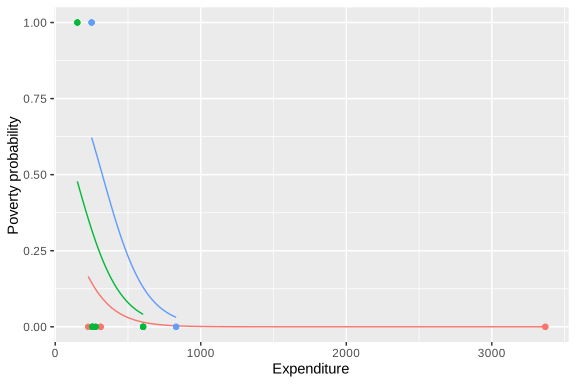
Figure 7.8: Predicted probability curves by stratum: logistic model with random intercept
7.4.3 Logistic Model with Random Intercept and Slope
The logistic model with random intercept and slope extends the previous specification by allowing not only the baseline level of the event to vary between strata, but also the effect of a specific covariate. This formulation is analogous to the random intercept and slope model for continuous variables, with the exception that the differences between strata are expressed on the logit scale and are translated into nonlinear probability curves.
Let \(x_{kj}\) be the covariate whose effect is allowed to vary between strata, and let \(\mathbf{z}_{kj}\) be the set of covariates with common fixed effects. In this model, the probability of success is assumed such that \(\text{logit}(\pi_{kj}) = \beta_{0j} + x_{kj}\beta_{1j} + \mathbf{z}_{kj}\boldsymbol{\beta}\). Here, \(\beta_{0j}\) is the stratum-specific intercept for stratum \(j\) and \(\beta_{1j}\) is the specific slope associated with the covariate \(x_{kj}\).
Both parameters are decomposed into a population-average part and a stratum-specific deviation, such that \(\beta_{0j} = \gamma_{00} + \tau_{0j}\) and \(\beta_{1j} = \gamma_{10} + \tau_{1j}\). The terms \(\gamma_{00}\) and \(\gamma_{10}\) represent, respectively, the global average intercept and the global average slope on a logit scale. For their part, \(\tau_{0j}\) and \(\tau_{1j}\) capture how much stratum \(j\) deviates from these averages. The implementation in R is as follows:
random_slope_logit_model <- glmer(
  poverty ~ 1 + Expenditure + (1 + Expenditure | Stratum),
  data = survey_data,
  weights = qk,
  family = binomial(link = "logit")
)
performance::icc(random_slope_logit_model)
## # Intraclass Correlation Coefficient
##
## Adjusted ICC: 0.875
## Unadjusted ICC: 0.631The estimation of the model with random intercept and slope indicates much more pronounced heterogeneity between strata. In this case, both the intercepts and slopes associated with expenditure can change between groups. The adjusted intraclass correlation is very high, suggesting that the between-strata component dominates the latent variation in the model. The model coefficients by stratum are shown in Table 7.7.
| (Intercept) | Expenditure | |
|---|---|---|
| idStrt001 | 4.865 | -0.025 |
| idStrt002 | 9.862 | -0.035 |
| idStrt003 | -1.133 | -0.007 |
| idStrt004 | 1.899 | -0.015 |
| idStrt005 | 8.030 | -0.026 |
| idStrt006 | -1.153 | 0.009 |
| idStrt007 | 0.974 | -0.012 |
| idStrt008 | 1.488 | -0.006 |
| idStrt009 | 3.660 | -0.005 |
| idStrt010 | 4.133 | -0.020 |
The coefficients by stratum show that the relationship between expenditure and poverty changes not only in its baseline level, but also in the strength and direction of the slope. In several strata the slope of expenditure is negative, which maintains the expected interpretation that higher levels of expenditure reduce the probability of poverty. However, slopes close to zero and even positive slopes also appear in some strata, suggesting distinct local patterns. This variability is precisely what the model seeks to capture through the random effect of the slope. Figure 7.9 shows that the predicted curves are more heterogeneous between strata than in the previous model:
prediction_data <- plot_data %>%
  group_by(Stratum) %>%
  summarise(
    Expenditure = list(seq(min(Expenditure), max(Expenditure), len = 100))
  ) %>%
  tidyr::unnest_legacy()

prediction_data <- prediction_data %>%
  mutate(
    probability = predict(
      random_slope_logit_model,
      newdata = prediction_data,
      type = "response"
    )
)ggplot(data = prediction_data,
aes(y = probability, x = Expenditure, colour = Stratum)) +
geom_line() +
geom_point(data = plot_data,
aes(y = poverty, x = Expenditure)) +
labs(y = "Poverty probability", x = "Expenditure") +
theme(legend.position = "none")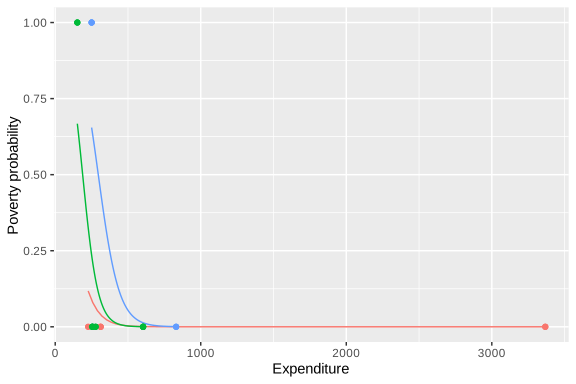
Figure 7.9: Predicted probability curves by stratum: logistic model with random intercept and slope