13.2 Definición del modelo
En muchas aplicaciones, la variable de interés en áreas pequeñas puede ser binaria, esto es \(y_{dj} = 0\) o \(1\) que representa la ausencia (o no) de una característica específica. Para este caso, la estimación objetivo en cada dominio \(d = 1,\cdots , D\) es la proporción \(\theta_d =\frac{1}{N_d}\sum_{i=1}^{N_d}y_{di}\) de la población que tiene esta característica, siendo \(\theta_{di}\) la probabilidad de que una determinada unidad \(i\) en el dominio \(d\) obtenga el valor \(1\). Bajo este escenario, el \(\theta_{di}\) con una función de enlace logit se define como:
\[ logit(\theta_{di}) = \log \left(\frac{\theta_{di}}{1-\theta_{di}}\right) = \boldsymbol{x}_{di}^{T}\boldsymbol{\beta} + u_{d} \] con \(i=1,\cdots,N_d\), \(d=1,\cdots,D\), \(\boldsymbol{\beta}\) un vector de parámetros de efecto fijo, y \(u_d\) el efecto aleatorio especifico del área para el dominio \(d\) con \(u_d \sim N\left(0,\sigma^2_u \right)\). \(u_d\) son independiente y \(y_{di}\mid u_d \sim Bernoulli(\theta_{di})\) con \(E(y_{di}\mid u_d)=\theta_{di}\) y \(Var(y_{di}\mid u_d)=\sigma_{di}^2=\theta_{di}(1-\theta_{di})\). Además, \(\boldsymbol{x}_{di}^T\) representa el vector \(p\times 1\) de valores de \(p\) variables auxiliares. Entonces, \(\theta_{di}\) se puede escribir como
\[ \theta_{di} = \frac{\exp(\boldsymbol{x}_{di}^T\boldsymbol{\beta} + u_{d})}{1+ \exp(\boldsymbol{x}_{di}^T\boldsymbol{\beta} + u_{d})} \] De está forma podemos definir distribuciones previas
\[ \begin{eqnarray*} \beta_k & \sim & N(0, 10000)\\ \sigma^2_u &\sim & IG(0.0001,0.0001) \end{eqnarray*} \] El modelo se debe estimar para cada una de las dimensiones.
Obejtivo
Estimar la proporción de personas que presentan la \(k-\)ésima carencia, es decir,
\[ P_d = \frac{\sum_{U_d}q_{di}}{N_d} \]
donde \(q_{di}\) toma el valor de 1 cuando la \(i-\)ésima persona presenta Privación Multidimensional y el valor de 0 en caso contrario.
Note que,
\[ \begin{equation*} \bar{Y}_d = P_d = \frac{\sum_{s_d}q_{di} + \sum_{s^c_d}q_{di}}{N_d} \end{equation*} \]
Ahora, el estimador de \(P\) esta dado por:
\[ \hat{P}_d = \frac{\sum_{s_d}q_{di} + \sum_{s^c_d}\hat{q}_{di}}{N_d} \]
donde
\[ \hat{q}_{di} = \frac{1}{8}\sum_{k=1}^{8}\hat{y}_{di}^{k} \]
\[\hat{y}_{di}^{k}=E_{\mathscr{M}}\left(y_{di}^{k}\mid\boldsymbol{x}_{d},\boldsymbol{\beta}\right)\],
con \(\mathscr{M}\) la medida de probabilidad inducida por el modelamiento. De esta forma se tiene que,
\[ \hat{P}_d = \frac{\sum_{U_{d}}\hat{q}_{di}}{N_d} \]
13.2.1 Procesamiento del modelo en R.
El proceso inicia con el cargue de las librerías.
library(patchwork)
library(lme4)
library(tidyverse)
library(rstan)
library(rstanarm)
library(magrittr)
Los datos de la encuesta y el censo han sido preparados previamente, la información sobre la cual realizaremos la predicción corresponde a Colombia en el 2019
encuesta_H <- readRDS("Recursos/Día4/Sesion3/Data/encuesta_ipm.rds")
statelevel_predictors_df <-
  readRDS("Recursos/Día4/Sesion3/Data/statelevel_predictors_df_dam2.rds") %>%
   mutate_at(.vars = c("luces_nocturnas",
                      "cubrimiento_cultivo",
                      "cubrimiento_urbano",
                      "modificacion_humana",
                      "accesibilidad_hospitales",
                      "accesibilidad_hosp_caminado"),
            function(x) as.numeric(scale(x)))

byAgrega <- c("dam", "dam2", "area", "sexo","anoest", "edad" )
names_H <- grep(pattern = "nbi", names(encuesta_H),value = TRUE)
encuesta_df <- map(setNames(names_H,names_H),
function(y){
encuesta_H$temp <- encuesta_H[[y]]
encuesta_H %>%
group_by_at(all_of(byAgrega)) %>%
summarise(n = n(),
yno = sum(temp),
ysi = n - yno, .groups = "drop") %>%
inner_join(statelevel_predictors_df)
})Privación en material de construcción de la vivienda
| dam | dam2 | area | sexo | anoest | edad | n | yno | ysi | modificacion_humana | accesibilidad_hospitales | accesibilidad_hosp_caminado | cubrimiento_cultivo | cubrimiento_urbano | luces_nocturnas | area1 | sexo2 | edad2 | edad3 | edad4 | edad5 | anoest2 | anoest3 | anoest4 | anoest99 | tiene_sanitario | tiene_acueducto | tiene_gas | eliminar_basura | tiene_internet | piso_tierra | material_paredes | material_techo | rezago_escolar | alfabeta | hacinamiento | tasa_desocupacion | id_municipio |
|---|---|---|---|---|---|---|---|---|---|---|---|---|---|---|---|---|---|---|---|---|---|---|---|---|---|---|---|---|---|---|---|---|---|---|---|---|---|
| 01 | 00101 | 1 | 1 | 3 | 2 | 652 | 27 | 625 | 3.6127 | -1.1835 | -1.5653 | -1.1560 | 7.2782 | 4.9650 | 1.0000 | 0.5224 | 0.2781 | 0.2117 | 0.1808 | 0.0725 | 0.2000 | 0.3680 | 0.2286 | 0.0193 | 0.0119 | 0.7946 | 0.0673 | 0.0810 | 0.6678 | 0.0033 | 0.0109 | 0.0111 | 0.3694 | 0.9247 | 0.1962 | 0.0066 | 100101 |
| 01 | 00101 | 1 | 2 | 3 | 2 | 624 | 24 | 600 | 3.6127 | -1.1835 | -1.5653 | -1.1560 | 7.2782 | 4.9650 | 1.0000 | 0.5224 | 0.2781 | 0.2117 | 0.1808 | 0.0725 | 0.2000 | 0.3680 | 0.2286 | 0.0193 | 0.0119 | 0.7946 | 0.0673 | 0.0810 | 0.6678 | 0.0033 | 0.0109 | 0.0111 | 0.3694 | 0.9247 | 0.1962 | 0.0066 | 100101 |
| 32 | 03201 | 1 | 2 | 3 | 2 | 575 | 22 | 553 | 2.7794 | -1.1311 | -1.4114 | -0.3529 | 4.1625 | 3.8009 | 0.9256 | 0.5173 | 0.2869 | 0.2158 | 0.1599 | 0.0502 | 0.2161 | 0.4041 | 0.1677 | 0.0161 | 0.0200 | 0.7131 | 0.0571 | 0.1791 | 0.7701 | 0.0102 | 0.0245 | 0.0153 | 0.2883 | 0.9252 | 0.1870 | 0.0074 | 103201 |
| 32 | 03201 | 1 | 1 | 3 | 2 | 547 | 39 | 508 | 2.7794 | -1.1311 | -1.4114 | -0.3529 | 4.1625 | 3.8009 | 0.9256 | 0.5173 | 0.2869 | 0.2158 | 0.1599 | 0.0502 | 0.2161 | 0.4041 | 0.1677 | 0.0161 | 0.0200 | 0.7131 | 0.0571 | 0.1791 | 0.7701 | 0.0102 | 0.0245 | 0.0153 | 0.2883 | 0.9252 | 0.1870 | 0.0074 | 103201 |
| 25 | 02501 | 1 | 1 | 3 | 2 | 505 | 25 | 480 | 1.4723 | -0.9237 | -1.0018 | 0.3619 | 1.3166 | 1.6641 | 0.8601 | 0.5084 | 0.2837 | 0.2250 | 0.1564 | 0.0596 | 0.2622 | 0.3832 | 0.1282 | 0.0114 | 0.0189 | 0.8665 | 0.1021 | 0.1307 | 0.7972 | 0.0134 | 0.0136 | 0.0160 | 0.2118 | 0.8939 | 0.1787 | 0.0044 | 012501 |
| 25 | 02501 | 1 | 2 | 3 | 2 | 447 | 15 | 432 | 1.4723 | -0.9237 | -1.0018 | 0.3619 | 1.3166 | 1.6641 | 0.8601 | 0.5084 | 0.2837 | 0.2250 | 0.1564 | 0.0596 | 0.2622 | 0.3832 | 0.1282 | 0.0114 | 0.0189 | 0.8665 | 0.1021 | 0.1307 | 0.7972 | 0.0134 | 0.0136 | 0.0160 | 0.2118 | 0.8939 | 0.1787 | 0.0044 | 012501 |
Hacinamiento
| dam | dam2 | area | sexo | anoest | edad | n | yno | ysi | modificacion_humana | accesibilidad_hospitales | accesibilidad_hosp_caminado | cubrimiento_cultivo | cubrimiento_urbano | luces_nocturnas | area1 | sexo2 | edad2 | edad3 | edad4 | edad5 | anoest2 | anoest3 | anoest4 | anoest99 | tiene_sanitario | tiene_acueducto | tiene_gas | eliminar_basura | tiene_internet | piso_tierra | material_paredes | material_techo | rezago_escolar | alfabeta | hacinamiento | tasa_desocupacion | id_municipio |
|---|---|---|---|---|---|---|---|---|---|---|---|---|---|---|---|---|---|---|---|---|---|---|---|---|---|---|---|---|---|---|---|---|---|---|---|---|---|
| 01 | 00101 | 1 | 1 | 3 | 2 | 652 | 221 | 431 | 3.6127 | -1.1835 | -1.5653 | -1.1560 | 7.2782 | 4.9650 | 1.0000 | 0.5224 | 0.2781 | 0.2117 | 0.1808 | 0.0725 | 0.2000 | 0.3680 | 0.2286 | 0.0193 | 0.0119 | 0.7946 | 0.0673 | 0.0810 | 0.6678 | 0.0033 | 0.0109 | 0.0111 | 0.3694 | 0.9247 | 0.1962 | 0.0066 | 100101 |
| 01 | 00101 | 1 | 2 | 3 | 2 | 624 | 207 | 417 | 3.6127 | -1.1835 | -1.5653 | -1.1560 | 7.2782 | 4.9650 | 1.0000 | 0.5224 | 0.2781 | 0.2117 | 0.1808 | 0.0725 | 0.2000 | 0.3680 | 0.2286 | 0.0193 | 0.0119 | 0.7946 | 0.0673 | 0.0810 | 0.6678 | 0.0033 | 0.0109 | 0.0111 | 0.3694 | 0.9247 | 0.1962 | 0.0066 | 100101 |
| 32 | 03201 | 1 | 2 | 3 | 2 | 575 | 181 | 394 | 2.7794 | -1.1311 | -1.4114 | -0.3529 | 4.1625 | 3.8009 | 0.9256 | 0.5173 | 0.2869 | 0.2158 | 0.1599 | 0.0502 | 0.2161 | 0.4041 | 0.1677 | 0.0161 | 0.0200 | 0.7131 | 0.0571 | 0.1791 | 0.7701 | 0.0102 | 0.0245 | 0.0153 | 0.2883 | 0.9252 | 0.1870 | 0.0074 | 103201 |
| 32 | 03201 | 1 | 1 | 3 | 2 | 547 | 167 | 380 | 2.7794 | -1.1311 | -1.4114 | -0.3529 | 4.1625 | 3.8009 | 0.9256 | 0.5173 | 0.2869 | 0.2158 | 0.1599 | 0.0502 | 0.2161 | 0.4041 | 0.1677 | 0.0161 | 0.0200 | 0.7131 | 0.0571 | 0.1791 | 0.7701 | 0.0102 | 0.0245 | 0.0153 | 0.2883 | 0.9252 | 0.1870 | 0.0074 | 103201 |
| 25 | 02501 | 1 | 1 | 3 | 2 | 505 | 101 | 404 | 1.4723 | -0.9237 | -1.0018 | 0.3619 | 1.3166 | 1.6641 | 0.8601 | 0.5084 | 0.2837 | 0.2250 | 0.1564 | 0.0596 | 0.2622 | 0.3832 | 0.1282 | 0.0114 | 0.0189 | 0.8665 | 0.1021 | 0.1307 | 0.7972 | 0.0134 | 0.0136 | 0.0160 | 0.2118 | 0.8939 | 0.1787 | 0.0044 | 012501 |
| 25 | 02501 | 1 | 2 | 3 | 2 | 447 | 89 | 358 | 1.4723 | -0.9237 | -1.0018 | 0.3619 | 1.3166 | 1.6641 | 0.8601 | 0.5084 | 0.2837 | 0.2250 | 0.1564 | 0.0596 | 0.2622 | 0.3832 | 0.1282 | 0.0114 | 0.0189 | 0.8665 | 0.1021 | 0.1307 | 0.7972 | 0.0134 | 0.0136 | 0.0160 | 0.2118 | 0.8939 | 0.1787 | 0.0044 | 012501 |
13.2.2 Definiendo el modelo multinivel.
Para cada dimensión que compone el H se ajusta el siguiente modelo mostrado en el script. En este código se incluye el uso de la función future_map que permite procesar en paralelo cada modelo O puede compilar cada por separado.
library(furrr)
library(rstanarm)
plan(multisession, workers = 4)

fit <- future_map(encuesta_df, function(xdat){
stan_glmer(
  cbind(yno, ysi) ~ (1 | dam2) +
    (1 | dam) +
    (1|edad) +
    area +
    (1|anoest) +
    sexo +
    tasa_desocupacion +
    luces_nocturnas +
    modificacion_humana,
  family = binomial(link = "logit"),
  data = xdat,
  cores = 7,
  chains = 4,
  iter = 300
)},
.progress = TRUE)

saveRDS(object = fit, "Recursos/Día4/Sesion3/Data/fits_H.rds")
Terminado la compilación de los modelos después de realizar validaciones sobre esto, pasamos hacer las predicciones en el censo.
13.2.3 Proceso de estimación y predicción
Los modelos fueron compilados de manera separada, por tanto, disponemos de un objeto .rds por cada dimensión del H
fit_agua <-
  readRDS(file = "Recursos/Día4/Sesion3/Data/fits_bayes_nbi_agua.rds")
fit_combustible <-
  readRDS(file = "Recursos/Día4/Sesion3/Data/fits_bayes_nbi_combus.rds")
fit_techo <-
  readRDS(file = "Recursos/Día4/Sesion3/Data/fits_bayes_nbi_techo.rds")
fit_energia <-
  readRDS(file = "Recursos/Día4/Sesion3/Data/fits_bayes_nbi_elect.rds")
fit_hacinamiento <-
  readRDS(file = "Recursos/Día4/Sesion3/Data/fits_bayes_nbi_hacina.rds")
fit_paredes <-
  readRDS(file = "Recursos/Día4/Sesion3/Data/fits_bayes_nbi_pared.rds")
fit_material <-
  readRDS(file = "Recursos/Día4/Sesion3/Data/fits_bayes_nbi_matviv.rds")
fit_saneamiento <-
  readRDS(file = "Recursos/Día4/Sesion3/Data/fits_bayes_nbi_saneamiento.rds")
Ahora, debemos leer la información del censo y crear los post-estrato
censo_H <- readRDS("Recursos/Día4/Sesion3/Data/censo_mrp_dam2.rds")

poststrat_df <- censo_H %>%
  group_by_at(byAgrega) %>%
  summarise(n = sum(n), .groups = "drop") %>%
  arrange(desc(n))
tba(head(poststrat_df))| dam | dam2 | area | sexo | anoest | edad | n |
|---|---|---|---|---|---|---|
| 32 | 03201 | 1 | 2 | 3 | 2 | 78858 |
| 32 | 03201 | 1 | 1 | 3 | 2 | 77566 |
| 01 | 00101 | 1 | 1 | 3 | 2 | 76098 |
| 01 | 00101 | 1 | 2 | 3 | 2 | 76002 |
| 25 | 02501 | 1 | 2 | 3 | 2 | 52770 |
| 25 | 02501 | 1 | 1 | 3 | 2 | 51227 |
Para realizar la predicción en el censo debemos incluir la información auxiliar
poststrat_df <- inner_join(poststrat_df, statelevel_predictors_df)
dim(poststrat_df)
## [1] 14120 36Para cada uno de los modelos anteriores debe tener las predicciones, para ejemplificar el proceso tomaremos el departamento de la Guajira de Colombia
- Privación de acceso al agua potable.
temp <- poststrat_df
epred_mat_agua <- posterior_epred(
  fit_agua,
  newdata = temp,
  type = "response",
  allow.new.levels = TRUE
)- Privación de acceso al combustible para cocinar.
epred_mat_combustible <-
  posterior_epred(
    fit_combustible,
    newdata = temp,
    type = "response",
    allow.new.levels = TRUE
)- Privación en material de los techo.
epred_mat_techo <-
  posterior_epred(
    fit_techo,
    newdata = temp,
    type = "response",
    allow.new.levels = TRUE
)- Acceso al servicio energía eléctrica.
epred_mat_energia <-
  posterior_epred(
    fit_energia,
    newdata = temp,
    type = "response",
    allow.new.levels = TRUE
)- Hacinamiento en el hogar.
epred_mat_hacinamiento <-
  posterior_epred(
    fit_hacinamiento,
    newdata = temp,
    type = "response",
    allow.new.levels = TRUE
)- Privación el material de las paredes.
epred_mat_paredes <-
  posterior_epred(
    fit_paredes,
    newdata = temp,
    type = "response",
    allow.new.levels = TRUE
)- Privación en material de construcción de la vivienda
epred_mat_material <-
  posterior_epred(
    fit_material,
    newdata = temp,
    type = "response",
    allow.new.levels = TRUE
)- Privación en saneamiento.
epred_mat_saneamiento <-
  posterior_epred(
    fit_saneamiento,
    newdata = temp,
    type = "response",
    allow.new.levels = TRUE
  )
Los resultados anteriores se deben procesarse en términos de carencia (1) y no carencia (0) para la \(k-esima\) dimensión .
- Privación de acceso al agua potable.
epred_mat_agua_dummy <-
  rbinom(n = nrow(epred_mat_agua) * ncol(epred_mat_agua) , 1,
         epred_mat_agua)

epred_mat_agua_dummy <- matrix(
  epred_mat_agua_dummy,
  nrow = nrow(epred_mat_agua),
  ncol = ncol(epred_mat_agua)
)- Privación de acceso al combustible para cocinar.
epred_mat_combustible_dummy <-
  rbinom(n = nrow(epred_mat_combustible) * ncol(epred_mat_combustible) ,
         1,
         epred_mat_combustible)

epred_mat_combustible_dummy <- matrix(
  epred_mat_combustible_dummy,
  nrow = nrow(epred_mat_combustible),
  ncol = ncol(epred_mat_combustible)
)- Acceso al servicio energía eléctrica
epred_mat_energia_dummy <-
  rbinom(n = nrow(epred_mat_energia) * ncol(epred_mat_energia) ,
         1,
         epred_mat_energia)

epred_mat_energia_dummy <- matrix(
  epred_mat_energia_dummy,
  nrow = nrow(epred_mat_energia),
  ncol = ncol(epred_mat_energia)
)- Hacinamiento en el hogar.
epred_mat_hacinamiento_dummy <-
  rbinom(
    n = nrow(epred_mat_hacinamiento) * ncol(epred_mat_hacinamiento) ,
    1,
    epred_mat_hacinamiento
  )

epred_mat_hacinamiento_dummy <-
  matrix(
    epred_mat_hacinamiento_dummy,
    nrow = nrow(epred_mat_hacinamiento),
    ncol = ncol(epred_mat_hacinamiento)
)- Privación el material de las paredes.
epred_mat_paredes_dummy <-
  rbinom(n = nrow(epred_mat_paredes) * ncol(epred_mat_paredes) ,
         1,
         epred_mat_paredes)

epred_mat_paredes_dummy <- matrix(
  epred_mat_paredes_dummy,
  nrow = nrow(epred_mat_paredes),
  ncol = ncol(epred_mat_paredes)
)- Privación en material de construcción de la vivienda
epred_mat_material_dummy <-
  rbinom(n = nrow(epred_mat_material) * ncol(epred_mat_material) ,
         1,
         epred_mat_material)

epred_mat_material_dummy <- matrix(
  epred_mat_material_dummy,
  nrow = nrow(epred_mat_material),
  ncol = ncol(epred_mat_material)
)- Privación en saneamiento.
epred_mat_saneamiento_dummy <-
  rbinom(n = nrow(epred_mat_saneamiento) * ncol(epred_mat_saneamiento) ,
         1,
         epred_mat_saneamiento)

epred_mat_saneamiento_dummy <- matrix(
  epred_mat_saneamiento_dummy,
  nrow = nrow(epred_mat_saneamiento),
  ncol = ncol(epred_mat_saneamiento)
)- Privación en material de los techo.
epred_mat_techo_dummy <-
  rbinom(n = nrow(epred_mat_techo) * ncol(epred_mat_techo) ,
         1,
         epred_mat_techo)

epred_mat_techo_dummy <- matrix(
  epred_mat_techo_dummy,
  nrow = nrow(epred_mat_techo),
  ncol = ncol(epred_mat_techo)
)
Con las variables dummy creadas es posible estimar el H
epred_mat_H <- (1/8) * (
  epred_mat_material_dummy +
    epred_mat_hacinamiento_dummy +
    epred_mat_agua_dummy +
    epred_mat_saneamiento_dummy +
    epred_mat_energia_dummy +
    epred_mat_paredes_dummy +
    epred_mat_combustible_dummy +
    epred_mat_techo_dummy)
Ahora, debemos dicotomizar la variable nuevamente.
epred_mat_H[epred_mat_H <= 0.4] <- 0
epred_mat_H[epred_mat_H != 0] <- 1
Finalmente realizamos el calculo del H así:
mean(colSums(t(epred_mat_H)*poststrat_df$n)/sum(poststrat_df$n))## [1] 0.008795743También es posible utilizar la función Aux_Agregado para las estimaciones.
Para obtener el resultado por municipio procedemos así:
source("Recursos/Día4/Sesion3/0Recursos/funciones_mrp.R")
mrp_estimate_dam2 <-
   Aux_Agregado(poststrat = temp,
                epredmat = epred_mat_H,
                byMap = "dam2")
tba(mrp_estimate_dam2 %>% head(10))| dam2 | mrp_estimate | mrp_estimate_se |
|---|---|---|
| 00101 | 0.0011 | 0.0056 |
| 00201 | 0.0010 | 0.0037 |
| 00202 | 0.0010 | 0.0039 |
| 00203 | 0.0143 | 0.0136 |
| 00204 | 0.0006 | 0.0034 |
| 00205 | 0.0002 | 0.0018 |
| 00206 | 0.0060 | 0.0117 |
| 00207 | 0.0072 | 0.0187 |
| 00208 | 0.0015 | 0.0054 |
| 00209 | 0.0024 | 0.0067 |
El siguiente paso es realizar el mapa de los resultados
library(sp)
library(sf)
library(tmap)

ShapeSAE <- read_sf("Shape/DOM_dam2.shp") %>%
 rename(dam2 = id_dominio) %>%
  mutate(dam2 = str_pad(
                 string = dam2,
                 width = 5,
                 pad = "0"
               ))
Los resultados nacionales son mostrados en el mapa.
brks_ing <- c(0,0.05,0.1,0.15, 0.20 ,0.3, 1)
maps3 <- tm_shape(ShapeSAE %>%
                    left_join(mrp_estimate_dam2,  by = "dam2"))

Mapa_ing3 <-
  maps3 + tm_polygons(
    "mrp_estimate",
    breaks = brks_ing,
    title = "H",
    palette = "YlOrRd",
    colorNA = "white"
  )

tmap_save(
  Mapa_ing3,
  "Recursos/Día4/Sesion3/Data/DOM_H.jpeg",
  width = 2000,
  height = 1500,
  asp = 0
)

Mapa_ing3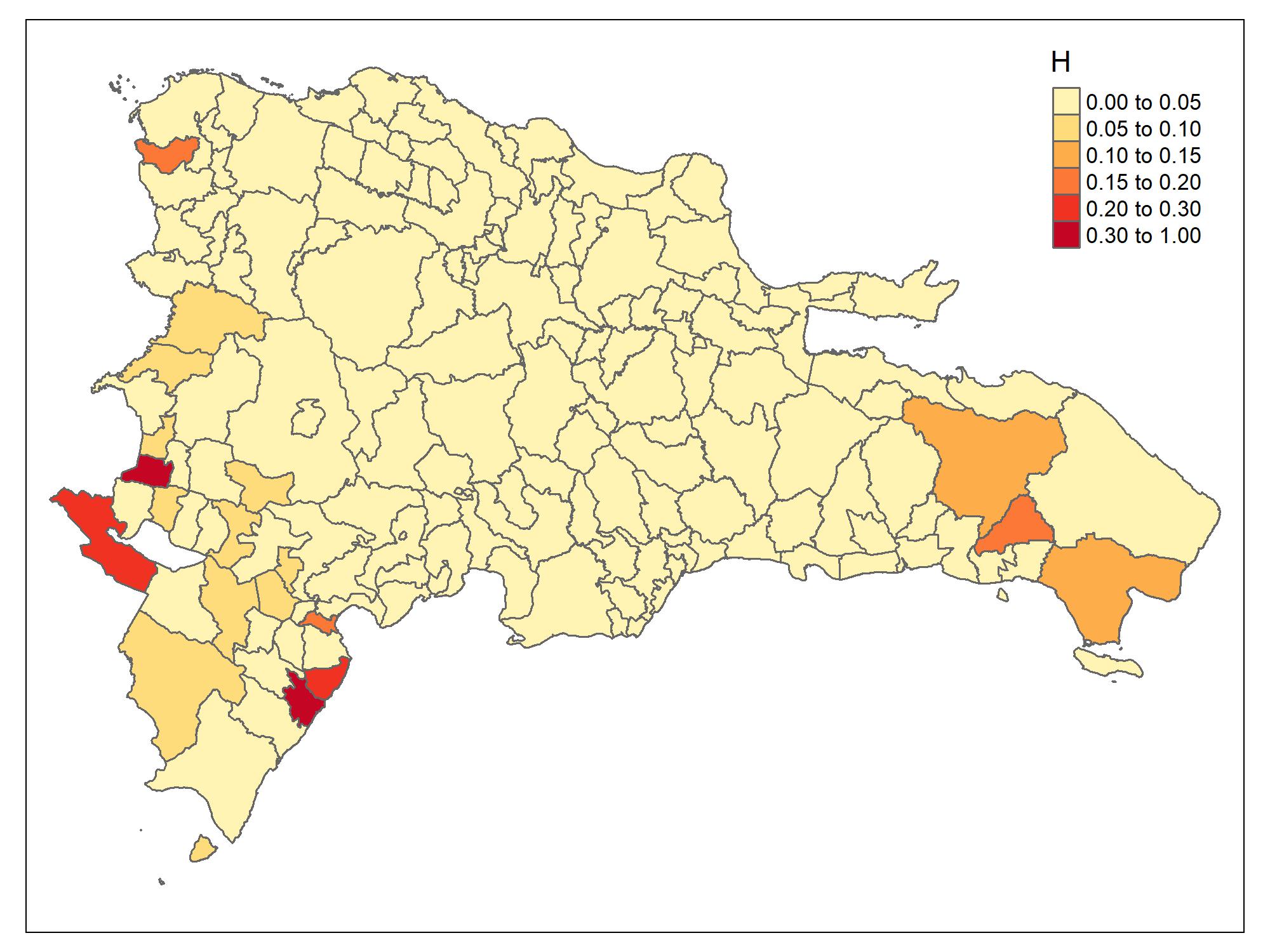
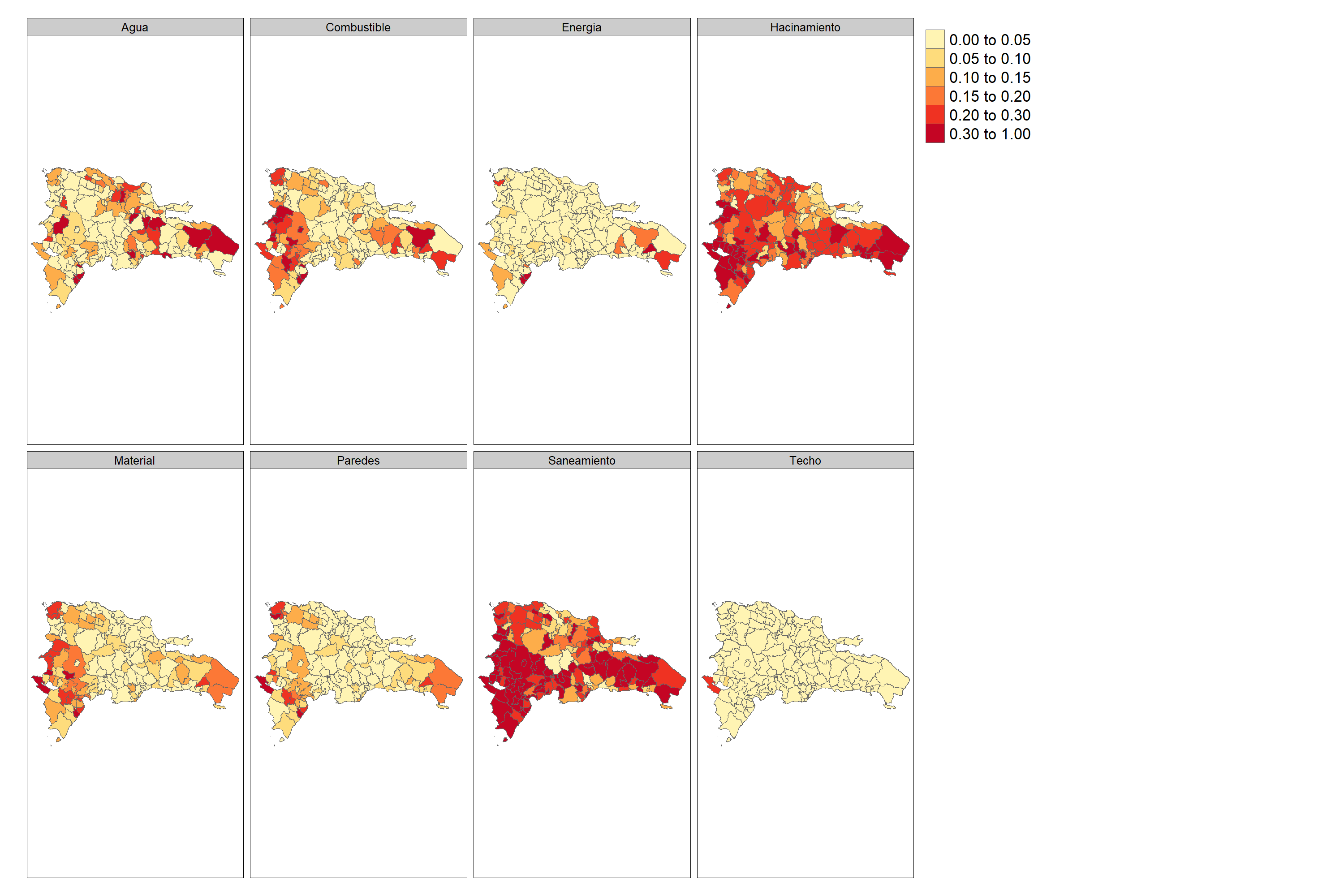
Los resultado para cada componente puede ser mapeado de forma similar.
Para obtener el resultado por municipio procedemos así:
| Indicador | dam2 | mrp_estimate |
|---|---|---|
| Material | 00101 | 0.0466 |
| Material | 00201 | 0.0337 |
| Material | 00202 | 0.0333 |
| Material | 00203 | 0.0562 |
| Material | 00204 | 0.0193 |
| Material | 00205 | 0.0148 |
| Material | 00206 | 0.0885 |
| Material | 00207 | 0.0746 |
| Material | 00208 | 0.0884 |
| Material | 00209 | 0.0430 |